Data Transformation and Exploratory Analysis
Task
Complete exercises from Data Transformation (chapter 3) and Exploratory Analysis (chapter 10) from Wickham et al (2017).
References
Wickham, H. (2017) R for data science: import, tidy, transform, visualise, and model data. Sebastopol, CA: O’Reilly Media.
Exercises, Chapter 3
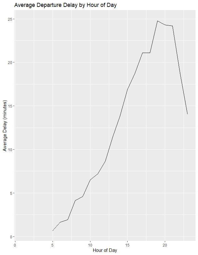
Figure 1. flight delay variation vary over the course of the day.
Flights were grouped by hour of expected departure and mean delay summarised before plot generated using geom_line
# Which carrier has the worst average delays? - answer frontier airlines

flights %>%
  summarise(delay = mean(dep_delay, na.rm = TRUE),
  .by = carrier)

 # Can you disentangle the effects of bad airports versus bad carriers?
#Why/why not? (Hint: Think about flights |> group_by(carrier, dest) |> summarize(n()).)

flights %>%
  summarise(delay = mean(dep_delay, na.rm = TRUE),
  n = n(),
  .by = c(carrier, dest))

#Find the flights that are most delayed upon departure from each destination.
flights %>%
  group_by(dest) %>%
  slice_max(dep_delay, n = 1, with_ties = FALSE) %>%
  relocate(dest)

 #How do delays vary over the course of the day. Illustrate your answer with a plot.
library(ggplot2)

delay_by_hour <- flights %>%
  group_by(hour) %>%
  summarise(delay = mean(dep_delay, na.rm = TRUE))

ggplot(delay_by_hour, aes(x = hour, y = delay)) +
  geom_line() +
  labs(
    title = "Average Departure Delay by Hour of Day",
    x = "Hour of Day",
    y = "Average Delay (minutes)")


#What happens if you supply a negative n to slice_min() and friends?
# assume it will take the 'opposite' - i.e. working the oppopsite direction.

flights %>%
  group_by(dest) %>%
  slice_max(dep_delay, n = -1, with_ties = FALSE) %>%
  relocate(dest)

# it actually seems to list all rows still so the slice does not work

# Explain what count() does in terms of the dplyr verbs you just learned. What does the sort argument to count() do?
flights |>
  group_by(month) |>
  count(sort= TRUE)

# count appears to count the number of rows in each group, description states it counts number of variables
# sort then orders them in descending order of n
flights %>%
  count(dest, sort = TRUE)

#Write down what you think the output of below df will look like;
#then check if you were correct and describe what group_by() does.
#alligned 1 to 5 to subsequent axis as predicted, group will creat two groups, a and b
#two groups shown in output # Groups:   y [2]. although df looks the same
#subsequent actions will be carried out on individual groups

df <- tibble(
  x = 1:5,
  y = c("a", "b", "a", "a", "b"),
  z = c("K", "K", "L", "L", "K")
)

df

df |>
  group_by(y)

#describe what arrange() does. Also comment on how it’s different from the group_by() in part (a).

#arrange will just put in order, df will look i.e. be shown with and then b, however the groups will not be formed and treated seperately in further actions
df |>
  arrange(y) # output as expected

#Write down what you think the output will look like; then check if you were correct and describe what the pipeline does.
# pipeline means, 'and then do': i.e. take what is before and then apply the result of this to the next function
df |>
  group_by(y) |>
  summarize(mean_x = mean(x)) #predict, groups by y and calculates mean of x for each group
#assumption was correct

df |>
  group_by(y, z) |>
  summarize(mean_x = mean(x)) # predict groups by y and then z and then summarises mean of resulting final groups
#prediction was correct

# how is output of below different to d?

df |>
  group_by(y, z) |>
  summarize(mean_x = mean(x), .groups = "drop")
# predict it ignores groups when calculating mean of x
# it did not drop groups..
# reading explained that it removed the groups after, so data no longer grouped
#if .groups=drop not included then the last grouping variable(z) is removed but other ones are kept.

df |>
  group_by(y, z) |>
  summarize(mean_x = mean(x))

df |>
  group_by(y, z) |>
  mutate(mean_x = mean(x))
Exercises - chapter 10
#Exercises
#1. improce visualisation of departure times of cancelled vs non cancelled flights.

flights |>
  mutate(
    cancelled = is.na(dep_time),
    sched_hour = sched_dep_time %/% 100,
    sched_min = sched_dep_time %% 100,
    sched_dep_time = sched_hour + (sched_min / 60)
  ) |>
  ggplot(aes(x = sched_dep_time, y = after_stat(density))) +
  geom_freqpoly(aes(color = cancelled), binwidth = 1/2, linewidth = 1)

#2  Based on EDA, what variable in the diamonds dataset appears to be most important for predicting the price of a diamond
# How is that variable correlated with cut?
# Why does the combination of those two relationships lead to lower-quality diamonds being more expensive?

?diamonds
ggplot(diamonds, aes(x=price, y = carat))+
  geom_point()+
  geom_smooth() # appears correlated

ggplot(diamonds, aes(x=price))+
  geom_freqpoly(aes(colour = color), binwidth 500, linewidth = 0.75))

ggplot(diamonds, aes(x=price, y = after_stat(density)))+
  geom_freqpoly(aes(colour = color), binwidth = 500, linewidth = 0.75) # no clear trend

ggplot(diamonds, aes(x=price, y = after_stat(density)))+
  geom_freqpoly(aes(colour = clarity), binwidth = 500, linewidth = 0.75) # some 'worse clarity' diamonds appear more expensive

#carat is the main predictor of price amoungst variables examined above

ggplot(diamonds, aes(x= carat, y = cut))+
  geom_boxplot() #poorer cut diamonds seem to be larger in terms of carats

ggplot(diamonds, aes(x=carat, y = after_stat(density)))+
  geom_freqpoly(aes(colour = cut), binwidth = 0.2, linewidth = 0.75) # confirms box plot, although maybe does not hold true for very large diamonds
#lower quality may be more expensive because they are larger diamonds in terms of carats

#3, use coord_flip() to switch axis, how different from specifying variables?
ggplot(diamonds, aes(x= carat, y = cut))+
  geom_boxplot()+
  coord_flip()

ggplot(diamonds, aes(x= cut, y = carat))+
  geom_boxplot() # they look the same

install.packages("lvplot")
library(lvplot)
ggplot(diamonds, aes(x= price, y = cut))+
  geom_boxplot()

ggplot(diamonds, aes(x = cut, y = price)) +
  geom_lv() +
  coord_flip() # see that more of most expensive diamonds are high quality, i.e the proportion of lower quality diamonds decreases as price increases

# Create a visualization of diamond prices versus a categorical variable from the diamonds dataset using geom_violin(),
# then a faceted geom_histogram(),
# then a colored geom_freqpoly(),
# and then a colored geom_density().
# Compare and contrast the four plots.
#What are the pros and cons of each method of visualizing the distribution of a numerical variable based on the levels of a categorical variable?

ggplot(diamonds, aes(x= clarity, y = price))+
  geom_violin() #provides info on distribution and frequency at each distribution but do not see small peaks or troughs

ggplot(diamonds, aes(x= price))+
  geom_histogram()+
    facet_grid(~clarity) # advantage that see shape of data in less smotthed manner, but graph is very busy


ggplot(diamonds, aes(x=price, y = after_stat(density)))+
  geom_freqpoly(aes(colour = clarity), binwidth = 500, linewidth = 0.75) # difficult to seperate differences by eye, smoothed plot gives overall shape but this may be effected by binwidth chosen


ggplot(diamonds, aes(x=price))+
  geom_density(aes(colour = clarity), linewidth = 0.75) # smoother graph and slightly better visualisation of overall trends than frequency polygon, but may loose some detail of bins that are larger or smaller than indicated by trend line

# Install/load packages
install.packages("ggbeeswarm")
library(ggplot2)
library(ggbeeswarm)


library(ggplot2)
library(ggbeeswarm)

# Beeswarm plot
p1 <- ggplot(diamonds, aes(x = cut, y = price)) +
  geom_beeswarm(aes(colour = cut)) +
  ggtitle("geom_beeswarm()")
p1

# Quasirandom plot
p2 <- ggplot(diamonds, aes(x = cut, y = price)) +
  geom_quasirandom(aes(colour = cut)) +
  ggtitle("geom_quasirandom()")

p2

# Display plots
library(gridExtra)
grid.arrange(p1, p2, p3, ncol = 1)


# two catgeorical values

ggplot(diamonds, aes(x = cut, y = color)) +
  geom_count()

#or compute counts with dplyr then visualis
diamonds |>
  count(color, cut)

diamonds |>
  count(color, cut) |>
  ggplot(aes(x = color, y = cut)) +
  geom_tile(aes(fill = n))

#exercises

diamonds %>% count(cut, color) %>%
  group_by(cut) %>%
  arrange(n, .by_group = TRUE)

#2 What different data insights do you get with a segmented bar chart if color is mapped to the x aesthetic and cut is mapped to the fill aesthetic?
#Calculate the counts that fall into each of the segments.

ggplot(diamonds, aes(x=color, fill = cut))+
  geom_bar()
#shows that proportion of different cuts seems to be similar across color


#Use geom_tile() together with dplyr to explore how average flight departure delays vary by destination and month of year.
#What makes the plot difficult to read? How could you improve it?

flights |>
  group_by(dest, month) %>%
  summarise(avg_delay = mean(dep_delay, na.rm = TRUE)) %>%
  ggplot(aes(x = factor(month), y = dest, fill = avg_delay)) + # added factor (month) as otherwise were not discrete values.
  geom_tile()
# the graph is too busy and there is no data for certain months.

# two numerical variables
ggplot(smaller, aes(x = carat, y = price)) +
  geom_point()
#could potentially be improved with an interactive plot so could select airport or region etc`.

# two numerical variables.

smaller <- diamonds |>
  filter(carat < 3)

ggplot(smaller, aes(x = carat, y = price)) +
  geom_point()

ggplot(smaller, aes(x = carat, y = price)) +
  geom_point(alpha = 1 / 100) # adds transparency, i do not like this as I think it hides data

# potential solution is to use bins  - geom_bin2d() and geom_hex() to bin in two dimensions.

ggplot(smaller, aes(x = carat, y = price)) +
  geom_bin2d()

# install.packages("hexbin")
ggplot(smaller, aes(x = carat, y = price)) +
  geom_hex()

#could also bin one variablem, e.g.

ggplot(smaller, aes(x = carat, y = price)) +
  geom_boxplot(aes(group = cut_width(carat, 0.1)))

# highlight number of data points by using varwidth = true
ggplot(smaller, aes(x = carat, y = price)) +
  geom_boxplot(aes(group = cut_width(carat, 0.1)), varwidth = TRUE)

#Exercises
# Fixed-width bins
smaller$carat_bin <- cut_width(smaller$carat, 0.1)

# Or bins with equal number of diamonds
smaller$carat_bin <- cut_number(smaller$carat, 10)

ggplot(smaller, aes(x = price, y = after_stat(density), group = carat_bin, color = carat_bin)) +
  geom_freqpoly(linewidth = 0.8)

# Visualize the distribution of carat, partitioned by price.
smaller$price_bin <- cut_width(smaller$price, 1000)
ggplot(smaller, aes(x=carat, y = after_stat(density), group = price_bin, colour = price_bin )) +
  geom_freqpoly(linewidth = 0.8)


diamonds %>%
  mutate(carat_bin = cut_width(carat, width = 1)) %>%
  ggplot(aes(x = price, colour = cut))+
  geom_freqpoly(binwidth = 500)+
  facet_wrap(cut~carat_bin)

  diamonds %>%
    mutate(price_bin = cut_width(price, width = 2000)) %>%
    ggplot(aes(x = carat, colour = cut)) +
    geom_freqpoly(binwidth = 0.1) +
    facet_wrap(~ price_bin)

  ggplot(diamonds, aes(x = price)) +
    geom_freqpoly(binwidth = 500, colour = "steelblue") +
    facet_grid(cut ~ color)


  diamonds %>%
    mutate(carat_bin = cut_width(carat, width = 1)) %>%
    ggplot(aes(x = price, colour = carat_bin)) +
    geom_freqpoly(binwidth = 500) +
    facet_wrap(~ cut) # this is what I wanted to do,
  #individual graphs are separated by cut,  carats are plotted by colour, price on x.

  diamonds %>%
    mutate(carat_bin = cut_width(carat, width = 0.5)) %>%
    ggplot(aes(x = price)) +
    geom_density() +
    facet_grid(cut ~ carat_bin)

  diamonds %>%
    mutate(price_bin = cut_width(price, width = 3000)) %>%
    ggplot(aes(x = carat)) +
    geom_density() +
    facet_grid(cut ~ price_bin)

 # 5, why is scatter better than binned for this case
  diamonds |>
    filter(x >= 4) |>
    ggplot(aes(x = x, y = y)) +
    geom_point() +
    coord_cartesian(xlim = c(4, 11), ylim = c(4, 11))
  # can see relationship between variables mor clearly and number of outliers, granularity is lost if data is binned

  #binned version
  diamonds %>%
    filter(x >= 4) %>%
    ggplot(aes(x = x, y = y)) +
    geom_bin2d() +
    coord_cartesian(xlim = c(4, 11), ylim = c(4, 11))