Classification methods
Task
Carry out the lab activities in the pages given below from the An Introduction to Statistical Learning with Applications in R textbook:
- 4.7 Lab: Classification Methods (Pages 171 – 177) - The Stock Market Data
- 8.3 Lab: Decision Trees (Pages 353 – 357).
Example graphs/data that were generated are shown below along with full coding.
References
James, G., Witten, D., Hastie, T. & Tibshirani, R., 2021. An Introduction to Statistical Learning: with Applications in R. 2nd ed. Springer, New York. doi:10.1007/978-1-0716-1418-1.
Logistic Regression.
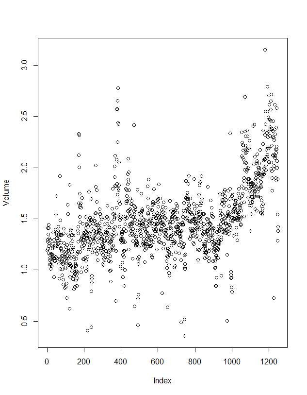
Figure 1. Scatter plot of raw data (coding shown below)
install.packages("ISLR2")
library(ISLR2)
data(Smarket)   # <— Load the dataset into the workspace
names(Smarket)
data(Smarket)
dim(Smarket)
summary(Smarket)

#cor() produces a matrix with all pairwise correlations among the predictors
cor(Smarket) # error because Direction is qualitative

cor(Smarket[, -9])  # corrleations are close to zero, except may be year/volume

attach(Smarket)
plot(Volume) # makes scatter plot (for this data type, different plot if different type) #Figure 1
View(Smarket)

#logistic regression
glm.fits <- glm(Direction ~ Lag1 + Lag2 + Lag3 + Lag4 + Lag5 + Volume, data = Smarket, family = binomial)
summary(glm.fits)

coef(glm.fits) # lists just the coefficients

summary(glm.fits)$coef # summary stats for coefficients


summary(glm.fits)$coef[, 4] # gives column 4, ie p values

# predict () predicts probability that market will go up given value of predictors,
# type = "response" tells R to output using P( Y=1|X ) rather than logit.
#if no data provided to predict(), then probs are computed for training data
# to find direction of probability use contrasts ()

glm.prob <- predict(glm.fits, type ="response")
glm.prob[1:10]

contrasts(Direction)

#convert probabilities in to class labels 'up' and 'down' based on if more or less than 0.5

glm.pred <- rep("Down", 1250) # makes vector of 1250 down elements
glm.pred[glm.prob >.5] = "Up" # makes all > 0. 5 "up"

#create confusion matrix to determing how many were correctly classified

table(glm.pred, Direction)

#percentage accurately predicted
(507+145)/1250 # 0.5216 = 52.2 percent

#however training error rate is often underestimated (page 175)
#better to split data and have a training and a test set for more realistic error rate

#create vector for data from 2001-2004 and keep 2005 as test data

train <- (Year < 2005)
Smarket.2005 <- Smarket[!train, ]
dim(Smarket.2005)

Direction.2005 <- Direction[!train]

#now fit logistic regression on 2001-2004 data using 'subset' argument
#then obtain predicted probs for 2005 (test set)

glm.fits <- glm(Direction ~ Lag1 + Lag2 + Lag3 + Lag4 + Lag5 + Volume, data = Smarket, family = binomial, subset = train)

glm.probs <- predict(glm.fits, Smarket.2005, type = "response")

# now table the predictions and actual results
glm.pred <- rep("Down", 252)
glm.pred[glm.probs >.5] = "Up"
table(glm.pred, Direction.2005)

> table(glm.pred, Direction.2005) #confusion matrix
        Direction.2005
glm.pred Down  Up
    Down   35  35
    Up     76 106
>

mean(glm.pred == Direction.2005)
mean(glm.pred != Direction.2005)  # this is the test set error, ie the prediction did not match the direction

# authors suggest refit with just Lag 1 and Lag2 as they had smallest p-values (although were still high)

glm.fits <- glm(Direction ~ Lag1 + Lag2, data = Smarket, family = binomial, subset = train)

glm.probs <- predict(glm.fits, Smarket.2005, type = "response")

glm.pred <- rep("Down", 252)
glm.pred[glm.probs > .5] <- "Up"

table(glm.pred, Direction.2005)

mean(glm.pred == Direction.2005)
mean(glm.pred != Direction.2005)

#if want to predict returns associated with specific values of Lag1 or Lag2
# ie predict Direction on dat where Lag 1 = 1.2 and Lag 2 = 1.1  and when = 1.5 and -0,8
# use predict() function

predict(glm.fits, newdata = data.frame(Lag1 = c(1.2, 1.5), Lag2 = c(1.1, -0.8)), type = "response")
Decision Trees
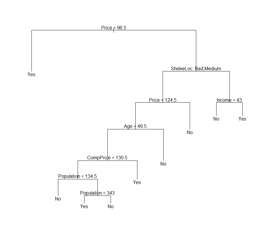
Figure 2. Example of generated deecision tree
install.packages("tree")

library(tree)

library(ISLR2)
attach(Carseats)
View(Carseats)

#going to convert sales (currently a continuous variable) to binary

High <- factor(ifelse(Sales <=8, "No", "Yes"))

#then use data.frame() to merge High with rest of the Carseats data
Carseats <- data.frame(Carseats, High)

View(Carseats)

#fit classification tree using all variables except Sales

tree.carseats <- tree(High ~ . -Sales, Carseats)

#summary lists variables used as internal nodes in tree, no. of nodes and training (error) rate

summary(tree.carseats) # see training error is 9%, 91% of observations correctly classified
#low residual mean devience is better but cant be interpreted well in isolation, maybe good for comparing with refined(pruned) tree models

#can graphically display the tree

#plot to display tree; test to display leaf nodes; pretty to include category names for qualitative predictors

plot(tree.carseats)
text(tree.carseats, pretty = 0)

#can get information on split criterion, number per brance, deviance etc as follows:
tree.carseats

# evaluate performance - need to estimate test error
# split into training and test set

#use predict() to evaluate performance on test data
#argument type = class instructs R to return actual class prediction

set.seed(2)
train <- sample(1:nrow(Carseats), 200)
Carseats.test <- Carseats[-train, ]
High.test <- High[-train]
tree.carseats <- tree(High ~ . - Sales, Carseats, subset = train)
tree.pred <- predict(tree.carseats, Carseats.test, type = "class")
table(tree.pred, High.test)

# does pruning tree improve the results?
#cv.tree performs cross validation
#use Fun = prune.misclass to state that want misclassification to guide the CV process rather than default of deviance

set.seed(7)
cv.carseats <- cv.tree(tree.carseats, FUN = prune.misclass)
names(cv.carseats)

cv.carseats #size is number of terminal nodes for each tree considered
#dev is corresponding error rate
#value of the cost-cost-complexity paramenter used (k)

#error rate is a function of size and k
par(mfrow = c (1,2))
plot(cv.carseats$size, cv.carseats$dev, type = "b")
plot(cv.carseats$k, cv.carseats$dev, type = "b")

#now prune tree obtain 9 node tree using prune.misclass()
prune.carseats <- prune.misclass(tree.carseats, best = 9)
plot(prune.carseats)
text(prune.carseats, pretty = 0)

#test pruned tree on dataset
tree.pred <- predict(prune.carseats, Carseats.test, type = "class")
table(tree.pred, High.test) #77.5 test observations correctly classified


# if increase value of best then obtain a larger pruned tree with lower classification accuracy

prune.carseats <- prune.misclass(tree.carseats, best = 14)
plot(prune.carseats)
text(prune.carseats, pretty = 0)
tree.pred <- predict(prune.carseats, Carseats.test, type = "class")
table(tree.pred, High.test)


#(could also use below to see which tree size gives lowest CV error)

best_index <- which.min(cv.carseats$dev)
best_index

# Exact values
cv.carseats$size[best_index]  # tree size with lowest deviance
cv.carseats$k[best_index]     # corresponding cost-complexity parameter k
cv.carseats$dev[best_index]   # the minimum deviance itself

#or put in a table
data.frame(
  size = cv.carseats$size[best_index],
  k    = cv.carseats$k[best_index],
  dev  = cv.carseats$dev[best_index]
)


# if increase value of best then obtain a larger pruned tree with lower classification accuracy


# 8.3.2 regression tree
attach(Boston)
set.seed(1)
train <- sample(1:nrow(Boston), nrow(Boston) / 2)
tree.Boston <- tree(medv ~., Boston, subset = train)
summary(tree.Boston)

#plot tree
plot(tree.Boston)
text(tree.Boston, pretty = 0)

#see if pruning the tree will improve performance
cv.boston <- cv.tree(tree.Boston)
plot(cv.boston$size, cv.boston$dev, type="b")

#most complex tree is selected by cross validation, but can test a pruned tree

prune.boston <- prune.tree(tree.Boston, best = 5)
plot(prune.boston)
text(prune.boston, pretty = 0)

#use unpruned tree to make predictions on test set
yhat <- predict(tree.Boston, newdata = Boston[-train, ])
boston.test <- Boston[-train, "medv"]
plot(yhat, boston.test)
abline(0, 1)
mean((yhat - boston.test)^2)

# MSE is 35.29, square root of MSE is 5.941 indicating the model leads to predictions on ave within
#  $5.941 of true median value

# useful to add proportion labels at the leaves?