Data Visualisation Activities in R

Task

Complete exercises from Data Visualisation (chapter 1) and Workflow Basics (chapter 2) from Wickham et al (2017).

Example graphs that were generated are shown below along with full coding.

References

Wickham, H. (2017) R for data science: import, tidy, transform, visualise, and model data. Sebastopol, CA: O’Reilly Media.

Learnings and Reflections

When aggregating data to make sure that not drawing assumptions based on a low number of data points, i.e some columns may have large amounts of missing data; it is important to explore the data before diving in to analysis.

Figure 1. Bar Graph illustrating penguin species found on each island.

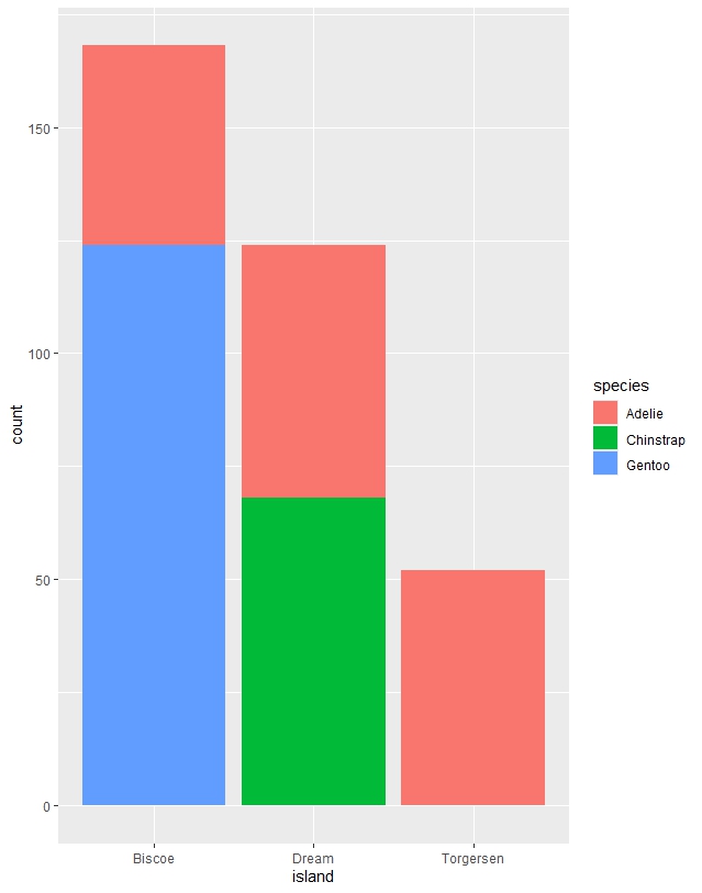
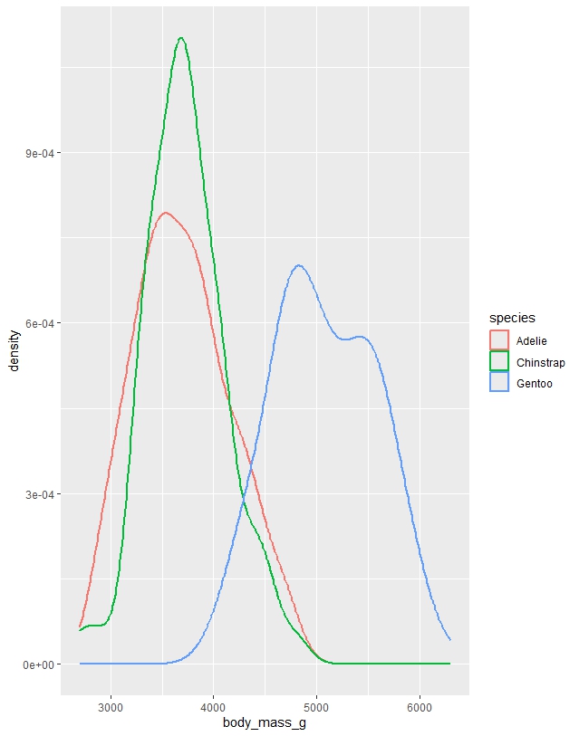
Bar graph - Penguins species per island

Figure 2. Density plot illustrating distribution of body weight by species.

Density plot - Penguin body weight

Chapter 1 Exercises

# Install and load required packages
install.packages("tidyverse")
library(tidyverse)

install.packages("palmerpenguins")
library(palmerpenguins)

install.packages("ggthemes")
library(ggthemes)

# View the dataset
penguins

# Open interactive data viewer
View(penguins)

# Open help page for the dataset
?penguins

# Create an empty plot (dataset only)
ggplot(data = penguins)

# Map variables to axes
ggplot(
  data = penguins,
  mapping = aes(x = flipper_length_mm, y = body_mass_g)
)

# Add points
ggplot(
  data = penguins,
  mapping = aes(x = flipper_length_mm, y = body_mass_g)
) +
  geom_point()

# Colour by species
ggplot(
  data = penguins,
  mapping = aes(
    x = flipper_length_mm,
    y = body_mass_g,
    colour = species
  )
) +
  geom_point()

# Add line of best fit (linear model)
ggplot(
  data = penguins,
  aes(
    x = flipper_length_mm,
    y = body_mass_g,
    colour = species
  )
) +
  geom_point() +
  geom_smooth(method = "lm")

# Single trend line (global vs local aesthetics)
ggplot(
  data = penguins,
  aes(x = flipper_length_mm, y = body_mass_g)
) +
  geom_point(aes(colour = species)) +
  geom_smooth(method = "lm")

# Add shapes for each species
ggplot(
  data = penguins,
  aes(x = flipper_length_mm, y = body_mass_g)
) +
  geom_point(aes(colour = species, shape = species)) +
  geom_smooth(method = "lm")

# Add labels and colour-blind friendly palette
ggplot(
  data = penguins,
  aes(x = flipper_length_mm, y = body_mass_g)
) +
  geom_point(aes(colour = species, shape = species)) +
  geom_smooth(method = "lm") +
  labs(
    title = "Body mass vs flipper length",
    subtitle = "Adelie, Chinstrap, and Gentoo penguins",
    x = "Flipper length (mm)",
    y = "Body mass (g)",
    colour = "Species",
    shape = "Species"
  ) +
  scale_color_colorblind()

# Dataset dimensions
nrow(penguins)
ncol(penguins)
dim(penguins)

# Scatterplot of bill length vs bill depth
ggplot(
  data = penguins,
  aes(x = bill_length_mm, y = bill_depth_mm)
) +
  geom_point()

# Scatterplot by species
ggplot(
  data = penguins,
  aes(x = species, y = bill_depth_mm)
) +
  geom_point()

# Handle missing values
ggplot(
  data = penguins,
  aes(x = species, y = bill_depth_mm)
) +
  geom_point(na.rm = TRUE)

# Add caption
ggplot(
  data = penguins,
  aes(x = species, y = bill_depth_mm)
) +
  geom_point(na.rm = TRUE) +
  labs(title = "Data from the palmerpenguins package")

# Histogram
ggplot(penguins, aes(x = body_mass_g)) +
  geom_histogram(binwidth = 200)

# Density plot
ggplot(penguins, aes(x = body_mass_g)) +
  geom_density()

# Boxplot
ggplot(
  penguins,
  aes(x = species, y = body_mass_g)
) +
  geom_boxplot()

# Stacked bar chart
ggplot(
  penguins,
  aes(x = island, fill = species)
) +
  geom_bar()

# Relative frequency
ggplot(
  penguins,
  aes(x = island, fill = species)
) +
  geom_bar(position = "fill")

# Faceting
ggplot(
  penguins,
  aes(x = flipper_length_mm, y = body_mass_g)
) +
  geom_point(aes(colour = species, shape = species)) +
  facet_wrap(~island)

# Save plot to disk
ggplot(
  penguins,
  aes(x = flipper_length_mm, y = body_mass_g)
) +
  geom_point()

ggsave("penguin-plot.png")

# Save most recent plot
ggplot(mpg, aes(x = class)) +
  geom_bar()

ggplot(mpg, aes(x = cty, y = hwy)) +
  geom_point()

ggsave("mpg-plot.png")

# Help for saving files
?ggsave

Chapter 2 Exercises

this_is_a_really_long_name <- 2.5
this_is_a_really_long_name
seq(from = 1, to = 10)
#can often omit names of first several aguements, i.e
seq(1, 10)
x <- "hello world"

# Exercises
#1. why does below code not work

my_variable <- 10
my_varıable

#answer, typo in calling my_variable

# 2 - correct below commands code
#libary(todyverse)

#ggplot(dTA = mpg) + 
#  geom_point(maping = aes(x = displ y = hwy)) +
#  geom_smooth(method = "lm)

library(tidyverse)

ggplot(data = mpg, mapping = aes(x = displ, y = hwy)) + 
  geom_point() +
  geom_smooth(method = "lm")

# 3. Press Option+Shift+K/Alt+Shift+K. What happens ? How get to same place using menus?

# this shows keyboard shortcut quick reference, also found under tool tab

# 4. run below code, which plot is saved as mpg-plot.png and why?

my_bar_plot <- ggplot(mpg, aes(x = class)) +
  geom_bar()
my_scatter_plot <- ggplot(mpg, aes(x = cty, y = hwy)) +
  geom_point()
ggsave(filename = "mpg-plot.png", plot = my_bar_plot)

#it saves the bar plot, because this has been specified in the argument?

⬅️ Return to Visualising Data