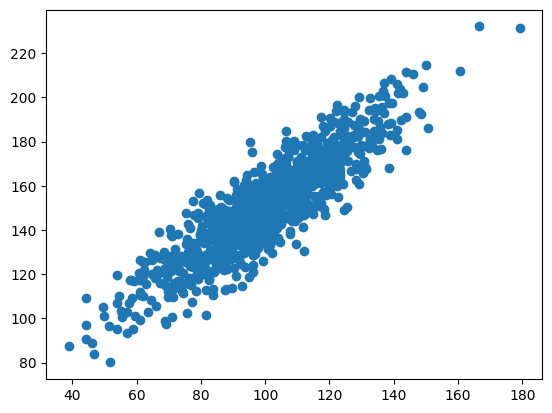
# calculate the Pearson's correlation between two variables
from numpy import mean
from numpy import std
from numpy import cov
from numpy.random import randn
from numpy.random import seed
from matplotlib import pyplot as plt
import seaborn as sns

from scipy.stats import pearsonr
# seed random number generator
seed(1)

# prepare data
data1 = 20 * randn(1000) + 100  # generating a 1000 reandom numbers with mean of 0 +100 and sd 20
data2 = data1 + (10 * randn(1000) + 50) # data 1 no plus second random number with mean 50 and sd 10 - result is that data is approx 50 more than data 1

# calculate covariance matrix
covariance = cov(data1, data2)

# calculate Pearson's correlation
corr, _ = pearsonr(data1, data2)

# plot
plt.scatter(data1, data2)
plt.show()

# summarize
print('data1: mean=%.3f stdv=%.3f' % (mean(data1), std(data1)))
print('data2: mean=%.3f stdv=%.3f' % (mean(data2), std(data2)))
print('Covariance: %.3f' % covariance[0][1])
print('Pearsons correlation: %.3f' % corr)

data1: mean=100.776 stdv=19.620
data2: mean=151.050 stdv=22.358
Covariance: 389.755
Pearsons correlation: 0.888

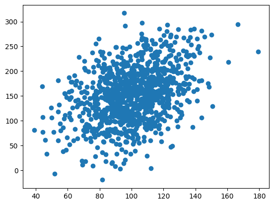
# changing the SD

from scipy.stats import pearsonr
# seed random number generator
seed(1)

# prepare data
data1 = 20 * randn(1000) + 100  # generating a 1000 reandom numbers with mean of 0 +100 and sd 20
data2 = data1 + (50 * randn(1000) + 50) # data 1 no plus second random number with mean 50 and sd 10 - result is that data is approx 50 more than data 1

# calculate covariance matrix
covariance = cov(data1, data2)

# calculate Pearson's correlation
corr, _ = pearsonr(data1, data2)

# plot
plt.scatter(data1, data2)
plt.show()

# summarize
print('data1: mean=%.3f stdv=%.3f' % (mean(data1), std(data1)))
print('data2: mean=%.3f stdv=%.3f' % (mean(data2), std(data2)))
print('Covariance: %.3f' % covariance[0][1])
print('Pearsons correlation: %.3f' % corr)

data1: mean=100.776 stdv=19.620
data2: mean=152.143 stdv=55.512
Covariance: 407.441
Pearsons correlation: 0.374

Increasing the SD made the data spread wider in the x axis for data1 variable and wider in the y axis for data2 variable; this is as expected as the variance and sd will increase. If the sd increases in both data1 and data2 together then the correlation decreases (again, as expected as the data points can vary more around the mean and are therefore less tightly constrained). If SD for data1 increases only then correlation becomes stronger, however if sd increases for y axis (data2) then the correlation is reduced (because this number is generated from data 1)

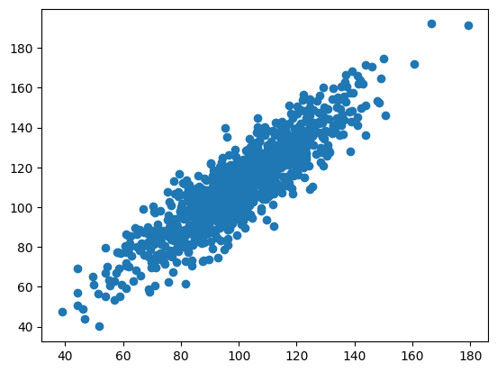
# change mean

from scipy.stats import pearsonr
# seed random number generator
seed(1)

# prepare data
data1 = 20 * randn(1000) + 100  # generating a 1000 reandom numbers with mean of 0 +100 and sd 20
data2 = data1 + (10 * randn(1000) + 10) # data 1 no plus second random number with mean 50 and sd 10 - result is that data is approx 50 more than data 1

# calculate covariance matrix
covariance = cov(data1, data2)

# calculate Pearson's correlation
corr, _ = pearsonr(data1, data2)

# plot
plt.scatter(data1, data2)
plt.show()

# summarize
print('data1: mean=%.3f stdv=%.3f' % (mean(data1), std(data1)))
print('data2: mean=%.3f stdv=%.3f' % (mean(data2), std(data2)))
print('Covariance: %.3f' % covariance[0][1])
print('Pearsons correlation: %.3f' % corr)

data1: mean=100.776 stdv=19.620
data2: mean=111.050 stdv=22.358
Covariance: 389.755
Pearsons correlation: 0.888

changing the mean shifts the dataset on the x or y axis, no effect on correlation, this is as expected as changing the mean value just shifts the data set around a different mean point.

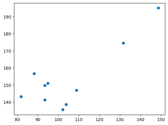
# change number of data points

from scipy.stats import pearsonr
# seed random number generator
seed(5)

# prepare data
data1 = 20 * randn(10) + 100  # generating a 1000 reandom numbers with mean of 0 +100 and sd 20
data2 = data1 + (10 * randn(10) + 50) # data 1 no plus second random number with mean 50 and sd 10 - result is that data is approx 50 more than data 1

# calculate covariance matrix
covariance = cov(data1, data2)

# calculate Pearson's correlation
corr, _ = pearsonr(data1, data2)

# plot
plt.scatter(data1, data2)
plt.show()

# summarize
print('data1: mean=%.3f stdv=%.3f' % (mean(data1), std(data1)))
print('data2: mean=%.3f stdv=%.3f' % (mean(data2), std(data2)))
print('Covariance: %.3f' % covariance[0][1])
print('Pearsons correlation: %.3f' % corr)

data1: mean=104.676 stdv=19.562
data2: mean=153.300 stdv=17.435
Covariance: 311.995
Pearsons correlation: 0.823

Changing the number of data points can effect the data shape and correlation value depending on seed given - Q how many data points do you need to be confident in the correlation value given, i.e. with 10 points and seed = 1,correlation = 0.971; but when seed = 5 correlation is 0.823 and despite coreelation coefficent suggesting a strong positive correlation, the graph above is not very convicing.