Unit 7 - Artificial Neural Networks

In the unit 7 lecturecast we learnt about the perceptron, a simple neural netowrk for binary classification. Working through relevent python exercises, it was possible to practice assigning input and weight values to a perceptron model, and to observe the effect on the output.

This notebook captures the multi-layer perceptron activity. In this notebook the step function is replaced with the sigmoid activation which, unlike a step function, enables gradient based learning through backpropagation. The sigmoid function however, has the disadvantage that it can become saturated across much of its domain, which makes gradient based learning difficult (Goodfellow et al, 2016). Despite this, sigmoid fuctions can be used to predict binary outputs.

Additional comments made to the original notebook have been indicated by initials ‘SJ’. These notes represent additional information for personal learning, observations and reflections which were made during completion of the exercise.

References

Goodfellow I, Bengio Y and Courville A. (2016) Deep Learning, Cambridge, MA: MIT Press. Available at: https://lccn.loc.gov/2016022992 (Accessed 05 June 2026).

Author: Dr Mike Lakoju

* If X is high, the value is approximately 1
* if X is small, the value is approximately 0

Import Libraries

import numpy as np

Define the Sigmoid Function

def sigmoid(sum_func):
  return 1 / (1 + np.exp(-sum_func))

SJ: The examples below show the output of applying the sigmoid function or np.exp (Eular’s number to the power of -sum_func) on various numbers. It can be seen that the sigmoid function transforms numbers on to a scale with values between 0 and 1.

sigmoid(0)

np.float64(0.5)

np.exp(2)

np.float64(7.38905609893065)

np.exp(1)

np.float64(2.718281828459045)

sigmoid(40)

np.float64(1.0)

sigmoid(-20.5)

np.float64(1.2501528648238605e-09)

Input Layer to Hidden Layer

Inputs

inputs = np.array([[0,0],
                   [0,1],
                   [1,0],
                   [1,1]])

inputs

array([[0, 0],
       [0, 1],
       [1, 0],
       [1, 1]])

inputs.shape

(4, 2)

Outputs

Output is considered ‘true’ only if either point is true (XOR)

outputs = np.array([[0],
                    [1],
                    [1],
                    [0]])

outputs.shape

(4, 1)

Weights

SJ: These weights are for the connection between the inputs and the hidden layer. The hidden layer has three neurons.

# First row holds the weights for x1, 2nd row contains the weights for x2

weights_0 = np.array([[-0.424, -0.740, -0.961],
                     [0.358, -0.577, -0.469]])
weights_0.shape

(2, 3)

These weights are for the connection between the hidden layer and the output

weights_1 = np.array([[-0.017],
                     [-0.893],
                     [0.148]])
weights_1.shape

(3, 1)

#### Epochs & Learning Rate

epochs = 100
learning_rate = 0.3

#for epoch in epochs:

input_layer = inputs
input_layer

array([[0, 0],
       [0, 1],
       [1, 0],
       [1, 1]])

# "sum_synapse_0" This holds the sum function total of weights for the hidden layer
# For the Output: Each row holds the sum_func for each input data  [0,0,0 -> data 0,0],[0.358, -0.577, -0.469 --> 0,1]
# The dot product does the matrix multiplication and also the sum

sum_synapse_0 = np.dot(input_layer, weights_0)
sum_synapse_0

array([[ 0.   ,  0.   ,  0.   ],
       [ 0.358, -0.577, -0.469],
       [-0.424, -0.74 , -0.961],
       [-0.066, -1.317, -1.43 ]])

SJ: The output array for sum_synapse_0 was initially confusing, breakdown of how the resulting matrix is generated is therefore shown in text.

This is the result of multiplying the imput layer (4 x 2 - x 1 and x 2, each which has 2 features) by the weights (2 x 3, as seen above and captures weight for each input to each hidden neuron)

i.e. for first row of sum_synapse_0 input = [0,0) to first hidden neuron: (0 * -0.424) + (0 * 0.358) = 0 + 0 = 0

input = [0,0) to second hidden neuron: (0 * -0.740) + (0 * -0.577) = 0 + 0 = 0`

input = [0,0) to third hidden neuron: 0 * -0.961) + (0 * -0.469) = 0 + 0 = 0

Which gives [0, 0, 0]

# Computing the Sigmoid function for the Hidden layer

hidden_layer = sigmoid(sum_synapse_0)
hidden_layer

array([[0.5       , 0.5       , 0.5       ],
       [0.5885562 , 0.35962319, 0.38485296],
       [0.39555998, 0.32300414, 0.27667802],
       [0.48350599, 0.21131785, 0.19309868]])

Dealing with the 2nd side

weights_1

array([[-0.017],
       [-0.893],
       [ 0.148]])

# "sum_synapse_1" This holds the sum function total of weights for the output layer
# For the Output: Each row holds the sum_func for each input data

sum_synapse_1 = np.dot(hidden_layer, weights_1)
sum_synapse_1

array([[-0.381     ],
       [-0.27419072],
       [-0.25421887],
       [-0.16834784]])

output_layer = sigmoid(sum_synapse_1)
output_layer

array([[0.40588573],
       [0.43187857],
       [0.43678536],
       [0.45801216]])

outputs

array([[0],
       [1],
       [1],
       [0]])

output_layer

array([[0.40588573],
       [0.43187857],
       [0.43678536],
       [0.45801216]])

error_output_layer = outputs - output_layer
error_output_layer

array([[-0.40588573],
       [ 0.56812143],
       [ 0.56321464],
       [-0.45801216]])

SJ: The error output above is the difference between the output layer and the expected outputs. As we can see, this untuned model is not able to correctly predict outputs.

average_error = np.mean(abs(error_output_layer))
average_error

np.float64(0.49880848923713045)

Sigmoid Derivative

def sigmoid_derivative(sigmoid):
    return sigmoid * (1 - sigmoid)

Delta output Calculation

# output_layer holds the results of our application of the sigmoid, computed above

output_layer

array([[0.40588573],
       [0.43187857],
       [0.43678536],
       [0.45801216]])

SJ: the derivative of the sigmoid function tells us the slope of the function at a particular point and therefore indicates the sensitivitiy of the output of a neuron to changes to the input. A steep slope means that small changes to the input will lead to larger changes in the output.

# derivative_output is our Derivative of the activation function (sigmoid) which we have on the slide
# each row is for each instance of our input dataset

derivative_output = sigmoid_derivative(output_layer)
derivative_output

array([[0.2411425 ],
       [0.24535947],
       [0.24600391],
       [0.24823702]])

error_output_layer

array([[-0.40588573],
       [ 0.56812143],
       [ 0.56321464],
       [-0.45801216]])

# Delta output
# each row is for each instance of our input dataset

delta_output = error_output_layer * derivative_output
delta_output

array([[-0.0978763 ],
       [ 0.13939397],
       [ 0.138553  ],
       [-0.11369557]])

Delta calculations for the Hidden Layer

delta_output

array([[-0.0978763 ],
       [ 0.13939397],
       [ 0.138553  ],
       [-0.11369557]])

weights_1

array([[-0.017],
       [-0.893],
       [ 0.148]])

NOTE THAT:

* Lets deal with this part first (Weight  * delta_output)
* Notice that we will get an error below becuase of the shape of the weights_1  (Transpose)

#delta_output_x_weight = delta_output.dot(weights_1)

weights_1.shape

(3, 1)

weights_1T = weights_1.T
weights_1T

array([[-0.017, -0.893,  0.148]])

weights_1T.shape

(1, 3)

Each one of the weights will have to be multiplied by each delta_output for each data instance

   array([[-0.017],
         [-0.893],
         [ 0.148]])

SJ: In the cell below, each row corresponds to each possible outcome (0,0: 0,1; 1,0; 1,1) and each column is for each hidden neuron. The resulting array is telling us the amount of error attributed to each hidden neuron for each input value.

delta_output_x_weight = delta_output.dot(weights_1T)
delta_output_x_weight

array([[ 0.0016639 ,  0.08740354, -0.01448569],
       [-0.0023697 , -0.12447882,  0.02063031],
       [-0.0023554 , -0.12372783,  0.02050584],
       [ 0.00193282,  0.10153015, -0.01682694]])

NOTE THAT:

* Now we need to deal with the last part of the equation   
* sigmoid_derivative * delta_output_x_weight

hidden_layer

array([[0.5       , 0.5       , 0.5       ],
       [0.5885562 , 0.35962319, 0.38485296],
       [0.39555998, 0.32300414, 0.27667802],
       [0.48350599, 0.21131785, 0.19309868]])

SJ: cell belöow is the error after taking in to account the hidden layers activation function,

#  Each row in the output of delta_hidden_layer is for the data input values

delta_hidden_layer = delta_output_x_weight * sigmoid_derivative(hidden_layer)
delta_hidden_layer

array([[ 0.00041597,  0.02185088, -0.00362142],
       [-0.00057384, -0.02866677,  0.00488404],
       [-0.00056316, -0.02705587,  0.00410378],
       [ 0.00048268,  0.01692128, -0.00262183]])

We will deal with the (input * delta) first

• The first column in “hidden_layer” holds the activation value for the first neuron

hidden_layer

array([[0.5       , 0.5       , 0.5       ],
       [0.5885562 , 0.35962319, 0.38485296],
       [0.39555998, 0.32300414, 0.27667802],
       [0.48350599, 0.21131785, 0.19309868]])

delta_output

array([[-0.0978763 ],
       [ 0.13939397],
       [ 0.138553  ],
       [-0.11369557]])

• We need to multiply the “inputs” by “delta” however, for the matrix multiplication we need to transpose the values in the hidden_layer, so we have all of them on one row for each neuron

hidden_layerT = hidden_layer.T
hidden_layerT

array([[0.5       , 0.5885562 , 0.39555998, 0.48350599],
       [0.5       , 0.35962319, 0.32300414, 0.21131785],
       [0.5       , 0.38485296, 0.27667802, 0.19309868]])

SJ: the cell below calculates the changes needed to the weights for the output layer.

input_x_delta1 = hidden_layerT.dot(delta_output)
input_x_delta1

array([[0.03293657],
       [0.02191844],
       [0.02108814]])

Let us now update the “weights_1”

SJ: calculates new weights from hidden to output layer

weights_1 = weights_1 + (input_x_delta1 * learning_rate)
weights_1

array([[-0.00711903],
       [-0.88642447],
       [ 0.15432644]])

Dealing with the Hidden Layer to Input Layer

# First column is X1, and 2nd column is X2 (our input values )

input_layer

array([[0, 0],
       [0, 1],
       [1, 0],
       [1, 1]])

delta_hidden_layer

array([[ 0.00041597,  0.02185088, -0.00362142],
       [-0.00057384, -0.02866677,  0.00488404],
       [-0.00056316, -0.02705587,  0.00410378],
       [ 0.00048268,  0.01692128, -0.00262183]])

# we need to transpose the values just as we did before

input_layerT = input_layer.T
input_layerT

array([[0, 0, 1, 1],
       [0, 1, 0, 1]])

input_x_delta0 = input_layerT.dot(delta_hidden_layer)
input_x_delta0

array([[-8.04778516e-05, -1.01345901e-02,  1.48194623e-03],
       [-9.11603819e-05, -1.17454886e-02,  2.26221011e-03]])

weights_0 = weights_0 + (input_x_delta0 * learning_rate)
weights_0

array([[-0.42402414, -0.74304038, -0.96055542],
       [ 0.35797265, -0.58052365, -0.46832134]])

So all the lines of code above, has allowed us to complete our first epoch. we will need to put all the code together so we can run multiple epochs

# Complete Artificial Neural Network

#Importing Numpy
import numpy as np

# This is the sigmoid Function
def sigmoid(sum):
  return 1 / (1 + np.exp(-sum))

#This is the sigmoid derivative as used before
def sigmoid_derivative(sigmoid):
  return sigmoid * (1 - sigmoid)

# Our input values
inputs = np.array([[0,0],
                   [0,1],
                   [1,0],
                   [1,1]])
#Our output values
outputs = np.array([[0],
                    [1],
                    [1],
                    [0]])

# weights_0 = np.array([[-0.424, -0.740, -0.961],
#                     [0.358, -0.577, -0.469]])

# weights_1 = np.array([[-0.017],
#                     [-0.893],
#                     [0.148]])

Initializing our weights with random values

• Note: Multiplying the random number by 2 and subtracting by 1, allows us to have a mix of both positive and negative random numbers for the weights

weights_0 = 2 * np.random.random((2, 3)) - 1
weights_1 = 2 * np.random.random((3, 1)) - 1

epochs = 400000
learning_rate = 0.6
error = []

for epoch in range(epochs):
  input_layer = inputs
  sum_synapse0 = np.dot(input_layer, weights_0)
  hidden_layer = sigmoid(sum_synapse0)

  sum_synapse1 = np.dot(hidden_layer, weights_1)
  output_layer = sigmoid(sum_synapse1)

  error_output_layer = outputs - output_layer
  average = np.mean(abs(error_output_layer))
    #print after every specified range of the value
  if epoch % 100000 == 0:
    print('Epoch: ' + str(epoch + 1) + ' Error: ' + str(average))
    error.append(average)

  derivative_output = sigmoid_derivative(output_layer)
  delta_output = error_output_layer * derivative_output

  weights1T = weights_1.T
  delta_output_weight = delta_output.dot(weights1T)
  delta_hidden_layer = delta_output_weight * sigmoid_derivative(hidden_layer)

  hidden_layerT = hidden_layer.T
  input_x_delta1 = hidden_layerT.dot(delta_output)
  weights_1 = weights_1 + (input_x_delta1 * learning_rate)

  input_layerT = input_layer.T
  input_x_delta0 = input_layerT.dot(delta_hidden_layer)
  weights_0 = weights_0 + (input_x_delta0 * learning_rate)

Epoch: 1 Error: 0.5006578575076446
Epoch: 100001 Error: 0.022270480968913677
Epoch: 200001 Error: 0.011966301414039919
Epoch: 300001 Error: 0.009125311306535353

At this point after runing for 1million epochs you can see the value is very low.

#1 million epochs with a learning rate of 0.3
1 - 0.009670967930930745

0.9903290320690693

#after 400,000 epochs, with a learning rate of 0.6
1- 0.008192022809586367

0.9918079771904136

Let’s visualize this result

import matplotlib.pyplot as plt

plt.xlabel('Number of Epochs')
plt.ylabel('Error')
plt.title('Plot showing results from Neural Network')
plt.plot(error)
plt.show()

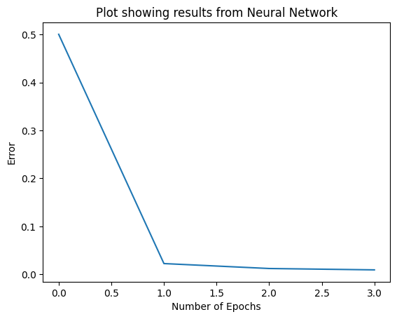
#### Comparing the outputs and the predictions

outputs

array([[0],
       [1],
       [1],
       [0]])

output_layer

array([[0.00834432],
       [0.99342966],
       [0.99342916],
       [0.00914117]])

* We see that our neural network was able to get values close to the actual values from the results.

* This shows that our neural network can handle the complexity of the XOR operator dataset.

• Let us see the updated weights. These are the weights we will require if we want to make future predictions

weights_0

array([[ -1.02866066, -12.88016741,   5.85527038],
       [ -1.02833672,   5.85954604, -12.86921948]])

weights_1

array([[-41.59319012],
       [ 16.02005006],
       [ 16.01754781]])

# This function accepts an instance of a dataset

def calculate_output(instance):
    #input to hidden layer
    hidden_layer = sigmoid(np.dot(instance, weights_0))
    #hidden to output layer
    output_layer = sigmoid(np.dot(hidden_layer, weights_1))
    return output_layer[0]

round(calculate_output(np.array([0, 0])))

0

round(calculate_output(np.array([0, 1])))

1

round(calculate_output(np.array([1, 0])))

1

round(calculate_output(np.array([1, 1])))

0