import pandas as pd
import numpy as npThis notebook presents my individual contributions to the data pre-processing and model development tasks undertaken for the Development Team Project, assessed in Unit 6. My colleague’s contributions — the random forest and linear regression models — are clearly marked with “Author: CF”; all other code in this notebook is my own work.
My collaborative contributions, including team leadership and document production, are addressed separately in the reflective essay
# 1. Load and Inspect Datasetdf = pd.read_csv("https://rossbulat.com/data/ab_nyc_2019.csv")df.info() # examine columns and data types; data types are as expected except last review (string cf datetime)
# neighbourhood group, neighbourhood and room type should be made to catagorical value (see later)<class 'pandas.core.frame.DataFrame'>
RangeIndex: 48895 entries, 0 to 48894
Data columns (total 16 columns):
# Column Non-Null Count Dtype
--- ------ -------------- -----
0 id 48895 non-null int64
1 name 48879 non-null object
2 host_id 48895 non-null int64
3 host_name 48874 non-null object
4 neighbourhood_group 48895 non-null object
5 neighbourhood 48895 non-null object
6 latitude 48895 non-null float64
7 longitude 48895 non-null float64
8 room_type 48895 non-null object
9 price 48895 non-null int64
10 minimum_nights 48895 non-null int64
11 number_of_reviews 48895 non-null int64
12 last_review 38843 non-null object
13 reviews_per_month 38843 non-null float64
14 calculated_host_listings_count 48895 non-null int64
15 availability_365 48895 non-null int64
dtypes: float64(3), int64(7), object(6)
memory usage: 6.0+ MBskewness = df.select_dtypes(include=np.number).skew().sort_values(ascending=False)
skewness| 0 | |
|---|---|
| minimum_nights | 21.827275 |
| price | 19.118939 |
| calculated_host_listings_count | 7.933174 |
| number_of_reviews | 3.690635 |
| reviews_per_month | 3.130189 |
| longitude | 1.284210 |
| host_id | 1.206214 |
| availability_365 | 0.763408 |
| latitude | 0.237167 |
| id | -0.090257 |
df.isnull().sum() # a large number of reviews per month are missing, do these correspond to number of reviews = 0 or just missing data?| 0 | |
|---|---|
| id | 0 |
| name | 16 |
| host_id | 0 |
| host_name | 21 |
| neighbourhood_group | 0 |
| neighbourhood | 0 |
| latitude | 0 |
| longitude | 0 |
| room_type | 0 |
| price | 0 |
| minimum_nights | 0 |
| number_of_reviews | 0 |
| last_review | 10052 |
| reviews_per_month | 10052 |
| calculated_host_listings_count | 0 |
| availability_365 | 0 |
# a large number of reviews per month are missing,
#do these correspond to number of reviews = 0 or  missing data?
missing_reviews = df[df["reviews_per_month"].isnull()]
missing_reviews["number_of_reviews"].value_counts().head(10)| count | |
|---|---|
| number_of_reviews | |
| 0 | 10052 |
#confirms that where reviews_per_month is missing it is because number of reviews = 0;
# therefore replace with 0df["reviews_per_month"] = df["reviews_per_month"].fillna(0)df.describe()| id | host_id | latitude | longitude | price | minimum_nights | number_of_reviews | reviews_per_month | calculated_host_listings_count | availability_365 | |
|---|---|---|---|---|---|---|---|---|---|---|
| count | 4.889500e+04 | 4.889500e+04 | 48895.000000 | 48895.000000 | 48895.000000 | 48895.000000 | 48895.000000 | 48895.000000 | 48895.000000 | 48895.000000 |
| mean | 1.901714e+07 | 6.762001e+07 | 40.728949 | -73.952170 | 152.720687 | 7.029962 | 23.274466 | 1.090910 | 7.143982 | 112.781327 |
| std | 1.098311e+07 | 7.861097e+07 | 0.054530 | 0.046157 | 240.154170 | 20.510550 | 44.550582 | 1.597283 | 32.952519 | 131.622289 |
| min | 2.539000e+03 | 2.438000e+03 | 40.499790 | -74.244420 | 0.000000 | 1.000000 | 0.000000 | 0.000000 | 1.000000 | 0.000000 |
| 25% | 9.471945e+06 | 7.822033e+06 | 40.690100 | -73.983070 | 69.000000 | 1.000000 | 1.000000 | 0.040000 | 1.000000 | 0.000000 |
| 50% | 1.967728e+07 | 3.079382e+07 | 40.723070 | -73.955680 | 106.000000 | 3.000000 | 5.000000 | 0.370000 | 1.000000 | 45.000000 |
| 75% | 2.915218e+07 | 1.074344e+08 | 40.763115 | -73.936275 | 175.000000 | 5.000000 | 24.000000 | 1.580000 | 2.000000 | 227.000000 |
| max | 3.648724e+07 | 2.743213e+08 | 40.913060 | -73.712990 | 10000.000000 | 1250.000000 | 629.000000 | 58.500000 | 327.000000 | 365.000000 |
# Examine price variable,# some listings have price = 0; how many?(df["price"] == 0).sum()np.int64(11)# as 11 have price == 0 this is very small percentage, therefore removedf = df[df["price"] > 0]#potential outliers in price (min and max), minimum nights (max).import matplotlib.pyplot as plt
plt.figure(figsize=(10, 5))
plt.boxplot(df['price'])
plt.title('Boxplot of Airbnb Prices')
plt.ylabel('Price')
plt.show()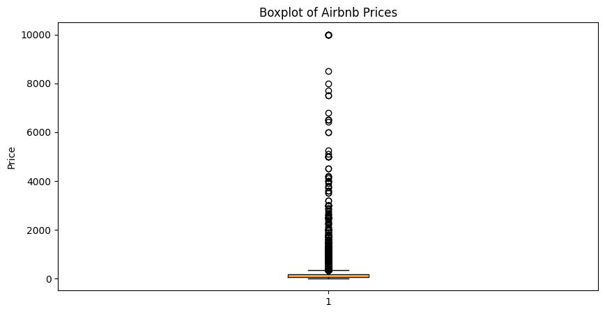
df["price"].describe(percentiles=[0.90, 0.95, 0.99])| price | |
|---|---|
| count | 48884.000000 |
| mean | 152.755053 |
| std | 240.170260 |
| min | 10.000000 |
| 50% | 106.000000 |
| 90% | 269.000000 |
| 95% | 355.000000 |
| 99% | 799.000000 |
| max | 10000.000000 |
df.sort_values(by="price", ascending=False)[
    ["name", "neighbourhood_group", "room_type", "price"]
].head(20)| name | neighbourhood_group | room_type | price | |
|---|---|---|---|---|
| 9151 | Furnished room in Astoria apartment | Queens | Private room | 10000 |
| 17692 | Luxury 1 bedroom apt. -stunning Manhattan views | Brooklyn | Entire home/apt | 10000 |
| 29238 | 1-BR Lincoln Center | Manhattan | Entire home/apt | 10000 |
| 12342 | Quiet, Clean, Lit @ LES & Chinatown | Manhattan | Private room | 9999 |
| 40433 | 2br - The Heart of NYC: Manhattans Lower East ... | Manhattan | Entire home/apt | 9999 |
| 6530 | Spanish Harlem Apt | Manhattan | Entire home/apt | 9999 |
| 30268 | Beautiful/Spacious 1 bed luxury flat-TriBeCa/Soho | Manhattan | Entire home/apt | 8500 |
| 4377 | Film Location | Brooklyn | Entire home/apt | 8000 |
| 29662 | East 72nd Townhouse by (Hidden by Airbnb) | Manhattan | Entire home/apt | 7703 |
| 45666 | Gem of east Flatbush | Brooklyn | Private room | 7500 |
| 42523 | 70' Luxury MotorYacht on the Hudson | Manhattan | Entire home/apt | 7500 |
| 44034 | 3000 sq ft daylight photo studio | Manhattan | Entire home/apt | 6800 |
| 48043 | Luxury TriBeCa Apartment at an amazing price | Manhattan | Entire home/apt | 6500 |
| 37194 | Apartment New York \nHell’s Kitchens | Manhattan | Private room | 6500 |
| 3774 | SUPER BOWL Brooklyn Duplex Apt!! | Brooklyn | Entire home/apt | 6500 |
| 29664 | Park Avenue Mansion by (Hidden by Airbnb) | Manhattan | Entire home/apt | 6419 |
| 15560 | Luxury townhouse Greenwich Village | Manhattan | Entire home/apt | 6000 |
| 3537 | UWS 1BR w/backyard + block from CP | Manhattan | Entire home/apt | 6000 |
| 3720 | SuperBowl Penthouse Loft 3,000 sqft | Manhattan | Entire home/apt | 5250 |
| 43009 | Midtown Manhattan great location (Gramacy park) | Manhattan | Entire home/apt | 5100 |
# these appear to be genuine data sets for luxury appartments, therefore retain and use a log transformation (price == 0 is already removed)
df["price_log"] = np.log1p(df["price"])
/tmp/ipykernel_3522/2910465958.py:2: SettingWithCopyWarning:
A value is trying to be set on a copy of a slice from a DataFrame.
Try using .loc[row_indexer,col_indexer] = value instead
See the caveats in the documentation: https://pandas.pydata.org/pandas-docs/stable/user_guide/indexing.html#returning-a-view-versus-a-copy
df["price_log"] = np.log1p(df["price"])# examine min nightsimport matplotlib.pyplot as plt
plt.figure(figsize=(10, 5))
plt.boxplot(df['minimum_nights'])
plt.title('Boxplot of minimum nights')
plt.ylabel('minimum nights')
plt.show()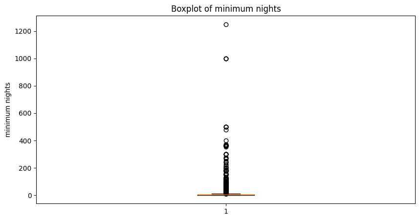
df["minimum_nights"].describe(percentiles=[0.90, 0.95, 0.99])| minimum_nights | |
|---|---|
| count | 48884.000000 |
| mean | 7.029887 |
| std | 20.512224 |
| min | 1.000000 |
| 50% | 3.000000 |
| 90% | 28.000000 |
| 95% | 30.000000 |
| 99% | 45.000000 |
| max | 1250.000000 |
# suggest have a cap at the 99th centile as these extreme values are likely to be outliers for various (unknown) reasonsupper_cap = df["minimum_nights"].quantile(0.99)
df["minimum_nights"] = np.where(
df["minimum_nights"] > upper_cap,
upper_cap,
df["minimum_nights"]
)/tmp/ipykernel_3522/3808001216.py:3: SettingWithCopyWarning:
A value is trying to be set on a copy of a slice from a DataFrame.
Try using .loc[row_indexer,col_indexer] = value instead
See the caveats in the documentation: https://pandas.pydata.org/pandas-docs/stable/user_guide/indexing.html#returning-a-view-versus-a-copy
df["minimum_nights"] = np.where(# examine availability
#note, we do not know exactly what this variable means (fully booked vs not available by host)
#therefore i think we should retain all data
(df["availability_365"] == 0).sum()np.int64(17530)plt.figure(figsize=(10, 5))
plt.boxplot(df['availability_365'])
plt.title('availability')
plt.ylabel('availability')
plt.show()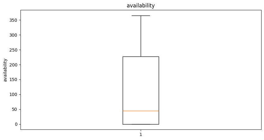
#given distribution and only mild skewness (see above) I would keep values as raw data. no further transformations required
# this is to preserve potential non linear effects and not lose patterns by grouping.df.describe(include='object') # examine non numberical data| name | host_name | neighbourhood_group | neighbourhood | room_type | last_review | |
|---|---|---|---|---|---|---|
| count | 48868 | 48863 | 48884 | 48884 | 48884 | 38833 |
| unique | 47894 | 11450 | 5 | 221 | 3 | 1764 |
| top | Hillside Hotel | Michael | Manhattan | Williamsburg | Entire home/apt | 2019-06-23 |
| freq | 18 | 417 | 21660 | 3919 | 25407 | 1412 |
# examine calculated_host_listings_count
# very skewed data set, no missing values.
# log trasnformdf["host_listings_log"] = np.log1p(
df["calculated_host_listings_count"]
)/tmp/ipykernel_3522/491388757.py:1: SettingWithCopyWarning:
A value is trying to be set on a copy of a slice from a DataFrame.
Try using .loc[row_indexer,col_indexer] = value instead
See the caveats in the documentation: https://pandas.pydata.org/pandas-docs/stable/user_guide/indexing.html#returning-a-view-versus-a-copy
df["host_listings_log"] = np.log1p(# examine longitude and latitude variablesdf[["latitude", "longitude"]].describe()| latitude | longitude | |
|---|---|---|
| count | 48884.000000 | 48884.000000 |
| mean | 40.728953 | -73.952176 |
| std | 0.054532 | 0.046159 |
| min | 40.499790 | -74.244420 |
| 25% | 40.690100 | -73.983080 |
| 50% | 40.723080 | -73.955685 |
| 75% | 40.763120 | -73.936290 |
| max | 40.913060 | -73.712990 |
import matplotlib.pyplot as plt # viewing distribution to check data spread (replica of graph Ross produced in the intro)

plt.scatter(df["longitude"], df["latitude"], s=1, alpha=0.3)
plt.title("Airbnb NYC Listings Spatial Distribution")
plt.xlabel("Longitude")
plt.ylabel("Latitude")
plt.show()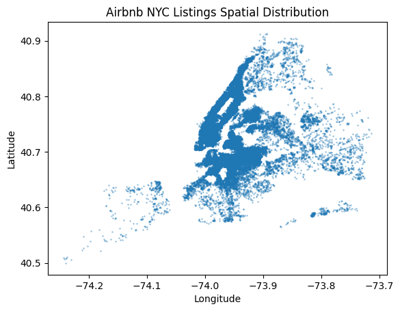
# these look as expected; no outliers found, no values missing as previously shown
# data can be used as is for scaling.
# Classify high demand properties as defined by Ross (i.e. top 25% of reviews_per_month)
df["high_demand"] = (df["reviews_per_month"] >= df["reviews_per_month"].quantile(0.75)).astype(int)/tmp/ipykernel_3522/934333795.py:2: SettingWithCopyWarning:
A value is trying to be set on a copy of a slice from a DataFrame.
Try using .loc[row_indexer,col_indexer] = value instead
See the caveats in the documentation: https://pandas.pydata.org/pandas-docs/stable/user_guide/indexing.html#returning-a-view-versus-a-copy
df["high_demand"] = (df["reviews_per_month"] >= df["reviews_per_month"].quantile(0.75)).astype(int)df["high_demand"].value_counts(normalize=True) # check of proportions for high demand. Look good!| proportion | |
|---|---|
| high_demand | |
| 0 | 0.748732 |
| 1 | 0.251268 |
df.groupby("neighbourhood_group")["high_demand"].mean() # just checking how the demand looks across neighbourhoods.| high_demand | |
|---|---|
| neighbourhood_group | |
| Bronx | 0.371560 |
| Brooklyn | 0.247375 |
| Manhattan | 0.220406 |
| Queens | 0.350688 |
| Staten Island | 0.391421 |
df.head()| id | name | host_id | host_name | neighbourhood_group | neighbourhood | latitude | longitude | room_type | price | minimum_nights | number_of_reviews | last_review | reviews_per_month | calculated_host_listings_count | availability_365 | price_log | host_listings_log | high_demand | |
|---|---|---|---|---|---|---|---|---|---|---|---|---|---|---|---|---|---|---|---|
| 0 | 2539 | Clean & quiet apt home by the park | 2787 | John | Brooklyn | Kensington | 40.64749 | -73.97237 | Private room | 149 | 1.0 | 9 | 2018-10-19 | 0.21 | 6 | 365 | 5.010635 | 1.945910 | 0 |
| 1 | 2595 | Skylit Midtown Castle | 2845 | Jennifer | Manhattan | Midtown | 40.75362 | -73.98377 | Entire home/apt | 225 | 1.0 | 45 | 2019-05-21 | 0.38 | 2 | 355 | 5.420535 | 1.098612 | 0 |
| 2 | 3647 | THE VILLAGE OF HARLEM....NEW YORK ! | 4632 | Elisabeth | Manhattan | Harlem | 40.80902 | -73.94190 | Private room | 150 | 3.0 | 0 | NaN | 0.00 | 1 | 365 | 5.017280 | 0.693147 | 0 |
| 3 | 3831 | Cozy Entire Floor of Brownstone | 4869 | LisaRoxanne | Brooklyn | Clinton Hill | 40.68514 | -73.95976 | Entire home/apt | 89 | 1.0 | 270 | 2019-07-05 | 4.64 | 1 | 194 | 4.499810 | 0.693147 | 1 |
| 4 | 5022 | Entire Apt: Spacious Studio/Loft by central park | 7192 | Laura | Manhattan | East Harlem | 40.79851 | -73.94399 | Entire home/apt | 80 | 10.0 | 9 | 2018-11-19 | 0.10 | 1 | 0 | 4.394449 | 0.693147 | 0 |
numeric_cols = [
    "price_log",
    "minimum_nights",
    "availability_365",
    "host_listings_log",
    "latitude",
    "longitude"
]
import seaborn as sns
import matplotlib.pyplot as plt

plt.figure(figsize=(8,6))
sns.heatmap(df[numeric_cols].corr(), annot=True, cmap="coolwarm")
plt.show()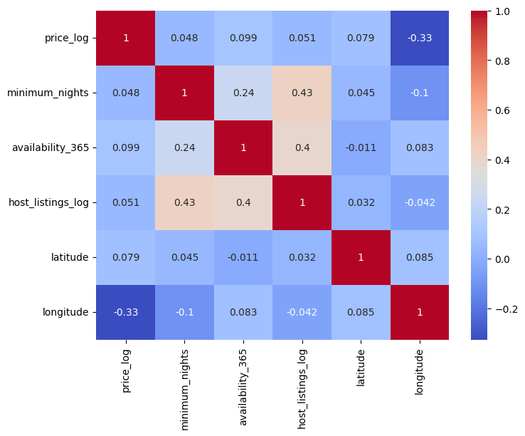
df.to_csv("airbnb_nyc_preprocessed.csv", index=False)import pandas as pd
import sklearn
print("Everything is installed")Everything is installedprint(df.columns.tolist())['id', 'name', 'host_id', 'host_name', 'neighbourhood_group', 'neighbourhood', 'latitude', 'longitude', 'room_type', 'price', 'minimum_nights', 'number_of_reviews', 'last_review', 'reviews_per_month', 'calculated_host_listings_count', 'availability_365', 'price_log', 'host_listings_log', 'high_demand']Model Comparison
Two classification models were evaluated for predicting high-demand Airbnb listings.
Logistic Regression
- Accuracy: 74.5%
- ROC-AUC: 0.738
Random Forest
- Accuracy: 81.0%
- ROC-AUC: 0.853
The Random Forest model substantially outperformed Logistic Regression across both evaluation metrics.
This suggests that the relationship between listing characteristics and demand is non-linear and involves complex feature interactions that are better captured by ensemble tree-based methods.
Random Forest is therefore selected as the stronger predictive model for this task.
Understanding the Features Drving Random Forest
Author: SJ
Adding availability_group to the DataFrame
bins = [0, 7, 30, 180, float('inf')]
labels = [1, 2, 3, 4]

df['availability_group'] = pd.cut(
    df['availability_365'],
    bins=bins,
    labels=labels,
    right=True,
    include_lowest=True
)

print(df['availability_group'].value_counts())
display(df.head())
#df.to_csv('/content/drive/MyDrive/airbnb_nyc_preprocessed_with_groups.csv', index=False)Random Forest Feature Importance Plot
import matplotlib.pyplot as plt
import seaborn as sns

# Get feature importances from the Random Forest model
feature_importances = rf_model.feature_importances_

# Get feature names from the training data
feature_names = X_train.columns

# Create a DataFrame for better visualization
importance_df = pd.DataFrame({
    'Feature': feature_names,
    'Importance': feature_importances
})

# Sort features by importance
importance_df = importance_df.sort_values(by='Importance', ascending=False)

# Plot the feature importances
plt.figure(figsize=(12, 8))
sns.barplot(x='Importance', y='Feature', data=importance_df, palette='viridis')
plt.title('Random Forest Feature Importance')
plt.xlabel('Importance Score')
plt.ylabel('Feature')
plt.tight_layout()
plt.show()
Impact of Top 5 Features on High Demand
import matplotlib.pyplot as plt
import seaborn as sns

# Get the top 5 most important features
top_5_features = importance_df['Feature'].head(5).tolist()

print(f"Top 5 features for analysis: {top_5_features}")

# Create subplots for each of the top 5 features
fig, axes = plt.subplots(nrows=5, ncols=1, figsize=(10, 25))
fig.suptitle('Distribution of Top 5 Features by High Demand Status', y=1.02, fontsize=16)

for i, feature in enumerate(top_5_features):
    sns.boxplot(x='high_demand', y=feature, data=df, ax=axes[i], palette='pastel')
    axes[i].set_title(f'Distribution of {feature} by High Demand')
    axes[i].set_xlabel('High Demand (0: No, 1: Yes)')
    axes[i].set_ylabel(feature)

plt.tight_layout()
plt.show()
Structured Neural Network Baseline
print(X_train.columns.tolist())['price_log', 'minimum_nights', 'availability_365', 'longitude', 'latitude', 'host_listings_log', 'neighbourhood_group_Brooklyn', 'neighbourhood_group_Manhattan', 'neighbourhood_group_Queens', 'neighbourhood_group_Staten Island', 'room_type_Private room', 'room_type_Shared room']import tensorflow as tf
from tensorflow import keras
from tensorflow.keras import layers
# Define the neural network architecture
# simple sequential model with a few dense layers
model = keras.Sequential([
# Input layer expects the number of features in X_train
layers.Input(shape=(X_train.shape[1],)),
layers.Dense(64, activation='relu'), # First hidden layer with 64 neurons and ReLU activation
layers.Dropout(0.2), # Dropout layer for regularization to prevent overfitting
layers.Dense(32, activation='relu'), # Second hidden layer with 32 neurons and ReLU activation
layers.Dropout(0.2), # Another dropout layer
layers.Dense(1, activation='sigmoid') # Output layer with 1 neuron and sigmoid activation for binary classification
])
# Compile the model
# Optimizer: Adam is a good general-purpose optimizer
# Loss: BinaryCrossentropy for binary classification problems
# Metrics: Accuracy to monitor performance during training
model.compile(
optimizer='adam',
loss='binary_crossentropy',
metrics=['accuracy']
)
# Display the model summary to see the layers and parameters
model.summary()Model: "sequential"
┏━━━━━━━━━━━━━━━━━━━━━━━━━━━━━━━━━┳━━━━━━━━━━━━━━━━━━━━━━━━┳━━━━━━━━━━━━━━━┓
┃ Layer (type)                    ┃ Output Shape           ┃       Param # ┃
┡━━━━━━━━━━━━━━━━━━━━━━━━━━━━━━━━━╇━━━━━━━━━━━━━━━━━━━━━━━━╇━━━━━━━━━━━━━━━┩
│ dense (Dense)                   │ (None, 64)             │           832 │
├─────────────────────────────────┼────────────────────────┼───────────────┤
│ dropout (Dropout)               │ (None, 64)             │             0 │
├─────────────────────────────────┼────────────────────────┼───────────────┤
│ dense_1 (Dense)                 │ (None, 32)             │         2,080 │
├─────────────────────────────────┼────────────────────────┼───────────────┤
│ dropout_1 (Dropout)             │ (None, 32)             │             0 │
├─────────────────────────────────┼────────────────────────┼───────────────┤
│ dense_2 (Dense)                 │ (None, 1)              │            33 │
└─────────────────────────────────┴────────────────────────┴───────────────┘
Total params: 2,945 (11.50 KB)
Trainable params: 2,945 (11.50 KB)
Non-trainable params: 0 (0.00 B)
Now that the model is defined and compiled, we can train it using the X_train and y_train data. We’ll also use a portion of the training data for validation to monitor performance and detect overfitting during the training process.
# Train the model
# epochs: number of times the model will iterate over the entire training dataset
# batch_size: number of samples per gradient update
# validation_split: percentage of training data to use for validation
history = model.fit(
    X_train,
    y_train,
    epochs=20,
    batch_size=32,
    validation_split=0.2, # Use 20% of the training data for validation
    verbose=1 # Show progress during training
)

print("\nNeural Network Training Complete!")
Epoch 1/20 978/978 ━━━━━━━━━━━━━━━━━━━━ 4s 3ms/step - accuracy: 0.7583 - loss: 0.4804 - val_accuracy: 0.7805 - val_loss: 0.4430 Epoch 2/20 978/978 ━━━━━━━━━━━━━━━━━━━━ 4s 4ms/step - accuracy: 0.7776 - loss: 0.4531 - val_accuracy: 0.7851 - val_loss: 0.4324 Epoch 3/20 978/978 ━━━━━━━━━━━━━━━━━━━━ 8s 7ms/step - accuracy: 0.7791 - loss: 0.4458 - val_accuracy: 0.7841 - val_loss: 0.4288 Epoch 4/20 978/978 ━━━━━━━━━━━━━━━━━━━━ 10s 10ms/step - accuracy: 0.7833 - loss: 0.4395 - val_accuracy: 0.7883 - val_loss: 0.4245 Epoch 5/20 978/978 ━━━━━━━━━━━━━━━━━━━━ 4s 4ms/step - accuracy: 0.7843 - loss: 0.4372 - val_accuracy: 0.7880 - val_loss: 0.4205 Epoch 6/20 978/978 ━━━━━━━━━━━━━━━━━━━━ 4s 4ms/step - accuracy: 0.7886 - loss: 0.4320 - val_accuracy: 0.7928 - val_loss: 0.4184 Epoch 7/20 978/978 ━━━━━━━━━━━━━━━━━━━━ 3s 3ms/step - accuracy: 0.7887 - loss: 0.4298 - val_accuracy: 0.7906 - val_loss: 0.4160 Epoch 8/20 978/978 ━━━━━━━━━━━━━━━━━━━━ 3s 3ms/step - accuracy: 0.7871 - loss: 0.4282 - val_accuracy: 0.7917 - val_loss: 0.4137 Epoch 9/20 978/978 ━━━━━━━━━━━━━━━━━━━━ 3s 3ms/step - accuracy: 0.7906 - loss: 0.4264 - val_accuracy: 0.7956 - val_loss: 0.4129 Epoch 10/20 978/978 ━━━━━━━━━━━━━━━━━━━━ 3s 3ms/step - accuracy: 0.7923 - loss: 0.4244 - val_accuracy: 0.7928 - val_loss: 0.4169 Epoch 11/20 978/978 ━━━━━━━━━━━━━━━━━━━━ 3s 3ms/step - accuracy: 0.7933 - loss: 0.4235 - val_accuracy: 0.7917 - val_loss: 0.4120 Epoch 12/20 978/978 ━━━━━━━━━━━━━━━━━━━━ 3s 3ms/step - accuracy: 0.7922 - loss: 0.4219 - val_accuracy: 0.7951 - val_loss: 0.4114 Epoch 13/20 978/978 ━━━━━━━━━━━━━━━━━━━━ 3s 3ms/step - accuracy: 0.7927 - loss: 0.4201 - val_accuracy: 0.7934 - val_loss: 0.4120 Epoch 14/20 978/978 ━━━━━━━━━━━━━━━━━━━━ 3s 3ms/step - accuracy: 0.7951 - loss: 0.4191 - val_accuracy: 0.7977 - val_loss: 0.4115 Epoch 15/20 978/978 ━━━━━━━━━━━━━━━━━━━━ 4s 4ms/step - accuracy: 0.7946 - loss: 0.4191 - val_accuracy: 0.7953 - val_loss: 0.4081 Epoch 16/20 978/978 ━━━━━━━━━━━━━━━━━━━━ 3s 3ms/step - accuracy: 0.7942 - loss: 0.4191 - val_accuracy: 0.7954 - val_loss: 0.4082 Epoch 17/20 978/978 ━━━━━━━━━━━━━━━━━━━━ 3s 3ms/step - accuracy: 0.7948 - loss: 0.4169 - val_accuracy: 0.7986 - val_loss: 0.4062 Epoch 18/20 978/978 ━━━━━━━━━━━━━━━━━━━━ 3s 3ms/step - accuracy: 0.7975 - loss: 0.4160 - val_accuracy: 0.7974 - val_loss: 0.4059 Epoch 19/20 978/978 ━━━━━━━━━━━━━━━━━━━━ 4s 4ms/step - accuracy: 0.7945 - loss: 0.4153 - val_accuracy: 0.7956 - val_loss: 0.4079 Epoch 20/20 978/978 ━━━━━━━━━━━━━━━━━━━━ 3s 3ms/step - accuracy: 0.7950 - loss: 0.4160 - val_accuracy: 0.7954 - val_loss: 0.4066 Neural Network Training Complete!
evaluate the model’s performance on the unseen X_test data
# Evaluate the model on the test set
loss, accuracy = model.evaluate(X_test, y_test, verbose=0)
print(f"Neural Network Test Accuracy: {accuracy:.4f}")

# Get predictions and probabilities for ROC-AUC
nn_pred_prob = model.predict(X_test)
nn_pred = (nn_pred_prob > 0.5).astype(int)

# Calculate ROC-AUC
roc_auc = roc_auc_score(y_test, nn_pred_prob)
print(f"Neural Network Test ROC-AUC: {roc_auc:.4f}")

# Print classification report and confusion matrix
print("\nClassification Report (Neural Network):")
print(classification_report(y_test, nn_pred))

print("\nConfusion Matrix (Neural Network):")
print(confusion_matrix(y_test, nn_pred))
Neural Network Test Accuracy: 0.7972 306/306 ━━━━━━━━━━━━━━━━━━━━ 0s 1ms/step Neural Network Test ROC-AUC: 0.8363 Classification Report (Neural Network): precision recall f1-score support 0 0.84 0.91 0.87 7333 1 0.63 0.46 0.53 2444 accuracy 0.80 9777 macro avg 0.73 0.69 0.70 9777 weighted avg 0.78 0.80 0.79 9777 Confusion Matrix (Neural Network): [[6658 675] [1308 1136]]
from sklearn.utils import class_weight
import numpy as np

# Calculate class weights
class_weights = class_weight.compute_class_weight(
    class_weight='balanced',
    classes=np.unique(y_train),
    y=y_train
)
class_weight_dict = dict(enumerate(class_weights))

print(f"Calculated Class Weights: {class_weight_dict}")
Calculated Class Weights: {0: np.float64(0.6680845975126418), 1: np.float64(1.98734627502795)}train the model with class_weights and Early Stopping enabled.
import tensorflow as tf
from tensorflow import keras
from tensorflow.keras import layers

# Define the Early Stopping callback
early_stopping = tf.keras.callbacks.EarlyStopping(
    monitor='val_loss', # Monitor the validation loss
    patience=5,         # Number of epochs with no improvement after which training will be stopped
    restore_best_weights=True # Restore model weights from the epoch with the best value of the monitored quantity
)

# Define the improved neural network architecture (same as the baseline for consistency, but a new instance)
model_improved = keras.Sequential([
    layers.Input(shape=(X_train.shape[1],)),
    layers.Dense(64, activation='relu'),
    layers.Dropout(0.2),
    layers.Dense(32, activation='relu'),
    layers.Dropout(0.2),
    layers.Dense(1, activation='sigmoid')
])

# Compile the improved model
model_improved.compile(
    optimizer='adam',
    loss='binary_crossentropy',
    metrics=['accuracy']
)

# Train the improved model with Early Stopping and Class Weights
history_improved = model_improved.fit(
    X_train,
    y_train,
    epochs=50, # Set a higher number of epochs, Early Stopping will prevent overfitting
    batch_size=32,
    validation_split=0.2,
    callbacks=[early_stopping], # Add the early stopping callback here
    class_weight=class_weight_dict, # Add class weights here
    verbose=1
)

print("\nImproved Neural Network Training Complete (with Class Weights)!")
Epoch 1/50 978/978 ━━━━━━━━━━━━━━━━━━━━ 5s 4ms/step - accuracy: 0.6922 - loss: 0.5828 - val_accuracy: 0.7130 - val_loss: 0.5525 Epoch 2/50 978/978 ━━━━━━━━━━━━━━━━━━━━ 3s 3ms/step - accuracy: 0.7170 - loss: 0.5414 - val_accuracy: 0.7290 - val_loss: 0.5413 Epoch 3/50 978/978 ━━━━━━━━━━━━━━━━━━━━ 3s 3ms/step - accuracy: 0.7249 - loss: 0.5326 - val_accuracy: 0.7370 - val_loss: 0.5158 Epoch 4/50 978/978 ━━━━━━━━━━━━━━━━━━━━ 4s 5ms/step - accuracy: 0.7305 - loss: 0.5240 - val_accuracy: 0.7407 - val_loss: 0.5087 Epoch 5/50 978/978 ━━━━━━━━━━━━━━━━━━━━ 3s 3ms/step - accuracy: 0.7322 - loss: 0.5178 - val_accuracy: 0.7396 - val_loss: 0.5058 Epoch 6/50 978/978 ━━━━━━━━━━━━━━━━━━━━ 3s 3ms/step - accuracy: 0.7349 - loss: 0.5160 - val_accuracy: 0.7446 - val_loss: 0.5134 Epoch 7/50 978/978 ━━━━━━━━━━━━━━━━━━━━ 3s 3ms/step - accuracy: 0.7382 - loss: 0.5115 - val_accuracy: 0.7324 - val_loss: 0.5494 Epoch 8/50 978/978 ━━━━━━━━━━━━━━━━━━━━ 4s 4ms/step - accuracy: 0.7406 - loss: 0.5098 - val_accuracy: 0.7580 - val_loss: 0.4889 Epoch 9/50 978/978 ━━━━━━━━━━━━━━━━━━━━ 4s 3ms/step - accuracy: 0.7408 - loss: 0.5081 - val_accuracy: 0.7480 - val_loss: 0.5070 Epoch 10/50 978/978 ━━━━━━━━━━━━━━━━━━━━ 3s 3ms/step - accuracy: 0.7450 - loss: 0.5035 - val_accuracy: 0.7453 - val_loss: 0.5251 Epoch 11/50 978/978 ━━━━━━━━━━━━━━━━━━━━ 3s 3ms/step - accuracy: 0.7449 - loss: 0.5038 - val_accuracy: 0.7403 - val_loss: 0.5233 Epoch 12/50 978/978 ━━━━━━━━━━━━━━━━━━━━ 4s 4ms/step - accuracy: 0.7465 - loss: 0.5008 - val_accuracy: 0.7464 - val_loss: 0.5217 Epoch 13/50 978/978 ━━━━━━━━━━━━━━━━━━━━ 3s 3ms/step - accuracy: 0.7504 - loss: 0.5000 - val_accuracy: 0.7552 - val_loss: 0.5052 Improved Neural Network Training Complete (with Class Weights)!
evaluate the performance of this new model.
# Evaluate the improved model on the test set
loss_improved, accuracy_improved = model_improved.evaluate(X_test, y_test, verbose=0)
print(f"Improved Neural Network Test Accuracy: {accuracy_improved:.4f}")

nn_pred_prob_improved = model_improved.predict(X_test)
nn_pred_improved = (nn_pred_prob_improved > 0.5).astype(int)

roc_auc_improved = roc_auc_score(y_test, nn_pred_prob_improved)
print(f"Improved Neural Network Test ROC-AUC: {roc_auc_improved:.4f}")

print("\nClassification Report (Improved Neural Network):")
print(classification_report(y_test, nn_pred_improved))

print("\nConfusion Matrix (Improved Neural Network):")
print(confusion_matrix(y_test, nn_pred_improved))
Improved Neural Network Test Accuracy: 0.7464 306/306 ━━━━━━━━━━━━━━━━━━━━ 2s 7ms/step Improved Neural Network Test ROC-AUC: 0.8276 Classification Report (Improved Neural Network): precision recall f1-score support 0 0.91 0.73 0.81 7333 1 0.50 0.79 0.61 2444 accuracy 0.75 9777 macro avg 0.70 0.76 0.71 9777 weighted avg 0.81 0.75 0.76 9777 Confusion Matrix (Improved Neural Network): [[5377 1956] [ 523 1921]]
Feature Importance for Improved Neural Network (Permutation Importance)
Since neural networks don’t have built-in feature_importances_ attributes like tree-based models, we’ll use Permutation Importance to understand which features are most influential in the model_improved.
from sklearn.inspection import permutation_importance
import matplotlib.pyplot as plt
import seaborn as sns
from sklearn.metrics import roc_auc_score
import tensorflow as tf
import numpy as np # Import numpy

# Create a wrapper class to make the Keras model compatible with sklearn's permutation_importance
class KerasClassifierWrapper:
    def __init__(self, keras_model):
        self.keras_model = keras_model
        self._estimator_type = 'classifier' # Explicitly declare as classifier
        self.classes_ = np.array([0, 1]) # Add the classes_ attribute for binary classification

    # permutation_importance expects a 'predict_proba' or 'decision_function' method
    # for probability-based scoring like 'roc_auc'. Keras models use .predict() for this.
    def predict_proba(self, X):
        # For binary classification, .predict() returns probabilities of the positive class (class 1)
        # We need to reshape it to (n_samples, 2) where the first column is prob of class 0
        # and the second column is prob of class 1.
        prob_class_1 = self.keras_model.predict(X, verbose=0).flatten()
        prob_class_0 = 1 - prob_class_1
        return np.vstack([prob_class_0, prob_class_1]).T

    # permutation_importance also checks for a 'fit' method, even if not explicitly used.
    # We'll provide a placeholder since our model is already trained.
    def fit(self, X, y):
        pass

# Wrap the improved Keras model
keras_wrapped_model = KerasClassifierWrapper(model_improved)

# Permutation importance for the improved neural network model
# We can now use 'roc_auc' directly because our wrapper provides predict_proba
result = permutation_importance(
    keras_wrapped_model, # Use the wrapped model
    X_test,
    y_test,
    scoring='roc_auc',
    n_repeats=10, # Number of times to permute a feature
    random_state=42,
    n_jobs=-1 # Use all available CPU cores
)

# Create a DataFrame for better visualization
perm_importance_df = pd.DataFrame({
    'Feature': X_test.columns,
    'Importance_Mean': result.importances_mean,
    'Importance_Std': result.importances_std
})

# Sort by importance mean
perm_importance_df = perm_importance_df.sort_values(by='Importance_Mean', ascending=False)

print("Permutation Feature Importance for Improved Neural Network (ROC-AUC):")
display(perm_importance_df)

# Plot the permutation importances
plt.figure(figsize=(12, 8))
sns.barplot(x='Importance_Mean', y='Feature', data=perm_importance_df, palette='viridis')
plt.title('Permutation Feature Importance')
plt.xlabel('Mean Decrease in ROC-AUC')
plt.ylabel('Feature')
plt.tight_layout()
plt.show()
Permutation Feature Importance for Improved Neural Network (ROC-AUC):| Feature | Importance_Mean | Importance_Std | |
|---|---|---|---|
| 2 | availability_365 | 0.179190 | 0.006861 |
| 1 | minimum_nights | 0.120145 | 0.003357 |
| 0 | price_log | 0.028996 | 0.001100 |
| 10 | room_type_Private room | 0.027389 | 0.001667 |
| 7 | neighbourhood_group_Manhattan | 0.026475 | 0.001845 |
| 5 | host_listings_log | 0.019965 | 0.001431 |
| 6 | neighbourhood_group_Brooklyn | 0.015669 | 0.001574 |
| 3 | longitude | 0.009947 | 0.001161 |
| 4 | latitude | 0.007490 | 0.000583 |
| 11 | room_type_Shared room | 0.006762 | 0.000929 |
| 8 | neighbourhood_group_Queens | 0.004842 | 0.000652 |
| 9 | neighbourhood_group_Staten Island | 0.000781 | 0.000206 |
/tmp/ipykernel_3522/2584035055.py:60: FutureWarning:

Passing `palette` without assigning `hue` is deprecated and will be removed in v0.14.0. Assign the `y` variable to `hue` and set `legend=False` for the same effect.

  sns.barplot(x='Importance_Mean', y='Feature', data=perm_importance_df, palette='viridis')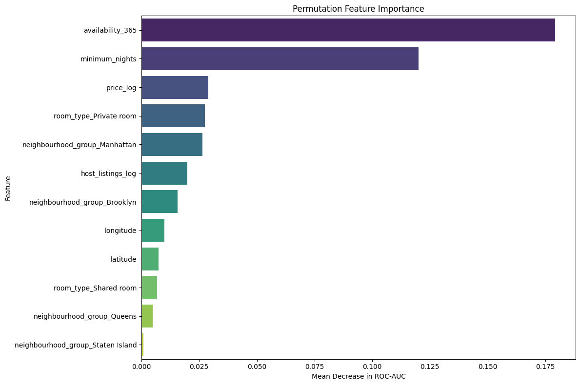
ROC Curve Analysis
Figure X shows the ROC curve for the improved neural network model. The model achieved a ROC-AUC score of 0.828, indicating good ability to distinguish between high-demand and non-high-demand listings. The curve lies well above the diagonal baseline, demonstrating performance substantially better than random classification. Given the class imbalance within the dataset, ROC-AUC provides a more informative measure of model performance than accuracy alone.
print(model_improved)nn_pred_prob_improved = model_improved.predict(X_test)
print(nn_pred_prob_improved[:5])from sklearn.metrics import average_precision_score
pr_auc_improved = average_precision_score(
y_test,
nn_pred_prob_improved
)
print(f"Improved Neural Network Test PR-AUC: {pr_auc_improved:.4f}")from sklearn.metrics import roc_auc_score, average_precision_score
loss_improved, accuracy_improved = model_improved.evaluate(
X_test, y_test, verbose=0
)
nn_pred_prob_improved = model_improved.predict(X_test)
roc_auc_improved = roc_auc_score(
y_test,
nn_pred_prob_improved
)
pr_auc_improved = average_precision_score(
y_test,
nn_pred_prob_improved
)
print(f"Accuracy: {accuracy_improved:.4f}")
print(f"ROC-AUC: {roc_auc_improved:.4f}")
print(f"PR-AUC: {pr_auc_improved:.4f}")from sklearn.metrics import roc_curve, roc_auc_score
import matplotlib.pyplot as plt
fpr, tpr, _ = roc_curve(y_test, nn_pred_prob_improved)
plt.figure(figsize=(6,5))
plt.plot(fpr, tpr, label=f'Improved Neural Network (AUC = {roc_auc_improved:.3f})')
plt.plot([0,1], [0,1], linestyle='--')
plt.xlabel('False Positive Rate')
plt.ylabel('True Positive Rate')
plt.title('ROC Curve - Improved Neural Network')
plt.legend()
plt.show()Analyzing Top Features for Business Insights
Now that we have the permutation importances, let’s look at the distributions of the top features against the high_demand target to suggest potential cut-offs for business insights.
import matplotlib.pyplot as plt
import seaborn as sns
import pandas as pd # Ensure pandas is imported

# Get the top 5 most important features based on permutation importance
top_5_perm_features = perm_importance_df['Feature'].head(5).tolist()

print(f"Top 5 features for cut-off analysis: {top_5_perm_features}")

# Construct plot_df by selectively getting features from df and X
plot_df_parts = {}
for feature in top_5_perm_features:
    if feature in df.columns: # Check if the feature is in the original df (likely numerical)
        plot_df_parts[feature] = df[feature]
    elif feature in X.columns: # Check if the feature is in the dummified X (likely one-hot encoded)
        plot_df_parts[feature] = X[feature]
    else:
        print(f"Warning: Feature '{feature}' not found in either df or X. Skipping.")

plot_df = pd.DataFrame(plot_df_parts)
plot_df['high_demand'] = y # Add the target variable

# Create subplots for each of the top 5 features
fig, axes = plt.subplots(nrows=len(top_5_perm_features), ncols=1, figsize=(10, 5 * len(top_5_perm_features)))
fig.suptitle('Distribution of Top Permutation Features by High Demand Status', y=1.02, fontsize=16)

for i, feature in enumerate(top_5_perm_features):
    ax = axes[i]
    # Check if the feature is numerical (not object, category, or boolean)
    if pd.api.types.is_numeric_dtype(plot_df[feature]) and not pd.api.types.is_bool_dtype(plot_df[feature]):
        # For numerical features, use boxplot
        sns.boxplot(x='high_demand', y=feature, data=plot_df, ax=ax, palette='pastel')
        ax.set_title(f'Distribution of {feature} by High Demand')
        ax.set_ylabel(feature)
    else:
        # For categorical or boolean features, use countplot
        sns.countplot(x=feature, hue='high_demand', data=plot_df, ax=ax, palette='pastel')
        ax.set_title(f'Count of {feature} by High Demand')
        ax.set_ylabel('Count')
    ax.set_xlabel('High Demand (0: No, 1: Yes)')

plt.tight_layout()
plt.show()

print("\n--- Business Insights & Potential Cut-offs ---")
for feature in top_5_perm_features:
    print(f"\nFeature: {feature}")
    if pd.api.types.is_numeric_dtype(plot_df[feature]) and not pd.api.types.is_bool_dtype(plot_df[feature]):
        high_demand_stats = plot_df[plot_df['high_demand'] == 1][feature].describe(percentiles=[0.25, 0.5, 0.75])
        low_demand_stats = plot_df[plot_df['high_demand'] == 0][feature].describe(percentiles=[0.25, 0.5, 0.75])
        print(f"  High Demand (1) Stats:\n{high_demand_stats}")
        print(f"  Low Demand (0) Stats:\n{low_demand_stats}")
        print(f"*Potential Cut-off Suggestion for {feature}*: Consider values where the distribution for 'high_demand=1' is distinctly different from 'high_demand=0'. For example, if the median/mean for 'high_demand=1' is much higher/lower than for 'high_demand=0'. This will be visually clearer in the box plots above.")
    else:
        cross_tab = plot_df.groupby([feature, 'high_demand']).size().unstack(fill_value=0)
        print(cross_tab)
        # Calculate percentages for high_demand=1
        if 1 in cross_tab.columns:
            cross_tab['Total'] = cross_tab[0] + cross_tab[1]
            cross_tab['% High Demand'] = (cross_tab[1] / cross_tab['Total'] * 100).round(2)
            print("\nPercentage of High Demand (1) for each category:")
            print(cross_tab[['% High Demand']])
        print(f"*Insight*: Examine categories with a higher proportion of `high_demand=1` listings.")
Top 5 features for cut-off analysis: ['availability_365', 'minimum_nights', 'price_log', 'room_type_Private room', 'neighbourhood_group_Manhattan']/tmp/ipykernel_3522/1424657933.py:32: FutureWarning:
Passing `palette` without assigning `hue` is deprecated and will be removed in v0.14.0. Assign the `x` variable to `hue` and set `legend=False` for the same effect.
sns.boxplot(x='high_demand', y=feature, data=plot_df, ax=ax, palette='pastel')
/tmp/ipykernel_3522/1424657933.py:32: FutureWarning:
Passing `palette` without assigning `hue` is deprecated and will be removed in v0.14.0. Assign the `x` variable to `hue` and set `legend=False` for the same effect.
sns.boxplot(x='high_demand', y=feature, data=plot_df, ax=ax, palette='pastel')
/tmp/ipykernel_3522/1424657933.py:32: FutureWarning:
Passing `palette` without assigning `hue` is deprecated and will be removed in v0.14.0. Assign the `x` variable to `hue` and set `legend=False` for the same effect.
sns.boxplot(x='high_demand', y=feature, data=plot_df, ax=ax, palette='pastel')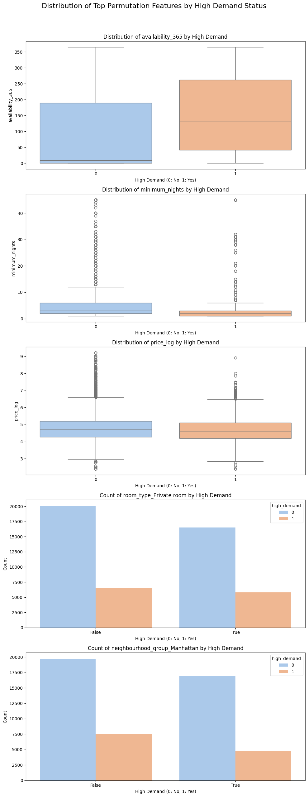
--- Business Insights & Potential Cut-offs ---

Feature: availability_365
  High Demand (1) Stats:
count    12283.000000
mean       151.542294
std        119.689782
min          0.000000
25%         41.000000
50%        131.000000
75%        262.000000
max        365.000000
Name: availability_365, dtype: float64
  Low Demand (0) Stats:
count    36601.000000
mean        99.771017
std        132.888979
min          0.000000
25%          0.000000
50%          9.000000
75%        189.000000
max        365.000000
Name: availability_365, dtype: float64
*Potential Cut-off Suggestion for availability_365*: Consider values where the distribution for 'high_demand=1' is distinctly different from 'high_demand=0'. For example, if the median/mean for 'high_demand=1' is much higher/lower than for 'high_demand=0'. This will be visually clearer in the box plots above.

Feature: minimum_nights
  High Demand (1) Stats:
count    12283.000000
mean         2.675975
std          4.093879
min          1.000000
25%          1.000000
50%          2.000000
75%          3.000000
max         45.000000
Name: minimum_nights, dtype: float64
  Low Demand (0) Stats:
count    36601.000000
mean         7.271085
std         10.159405
min          1.000000
25%          2.000000
50%          3.000000
75%          6.000000
max         45.000000
Name: minimum_nights, dtype: float64
*Potential Cut-off Suggestion for minimum_nights*: Consider values where the distribution for 'high_demand=1' is distinctly different from 'high_demand=0'. For example, if the median/mean for 'high_demand=1' is much higher/lower than for 'high_demand=0'. This will be visually clearer in the box plots above.

Feature: price_log
  High Demand (1) Stats:
count    12283.000000
mean         4.685380
std          0.640101
min          2.397895
25%          4.189655
50%          4.615121
75%          5.105945
max          8.922792
Name: price_log, dtype: float64
  Low Demand (0) Stats:
count    36601.000000
mean         4.755593
std          0.707414
min          2.397895
25%          4.262680
50%          4.709530
75%          5.198497
max          9.210440
Name: price_log, dtype: float64
*Potential Cut-off Suggestion for price_log*: Consider values where the distribution for 'high_demand=1' is distinctly different from 'high_demand=0'. For example, if the median/mean for 'high_demand=1' is much higher/lower than for 'high_demand=0'. This will be visually clearer in the box plots above.

Feature: room_type_Private room
high_demand                 0     1
room_type_Private room
False                   20071  6494
True                    16530  5789

Percentage of High Demand (1) for each category:
high_demand             % High Demand
room_type_Private room
False                           24.45
True                            25.94
*Insight*: Examine categories with a higher proportion of `high_demand=1` listings.

Feature: neighbourhood_group_Manhattan
high_demand                        0     1
neighbourhood_group_Manhattan
False                          19715  7509
True                           16886  4774

Percentage of High Demand (1) for each category:
high_demand                    % High Demand
neighbourhood_group_Manhattan
False                                  27.58
True                                   22.04
*Insight*: Examine categories with a higher proportion of `high_demand=1` listings.